Budget Optimisation

Use PanelBudgetOptimizerWrapper when you want to optimise spend for a fitted PanelMMM over a future date window.

The wrapper rejects the named FE, CRE and release-gated RE presets with EstimatorOperationError. Use the estimator support matrix before preparing an optimisation. FE/CRE historical and manual scenarios are separate supported operations; they do not enable fixed-budget optimisation.

The wrapper builds a synthetic future dataset for the requested window, swaps the model’s channel_data for an optimisation variable, and then calls the generic BudgetOptimizer. If you want to compare several plans in total horizon spend units, see Scenario Planning.

What the optimiser maximises

For PanelBudgetOptimizerWrapper, optimize_budget() defaults to:

• response_variable="total_media_contribution_original_scale"
• utility_function=average_response
• SciPy SLSQP with ftol=1e-9 and maxiter=1000

The optimiser therefore maximises the average posterior response of the chosen response variable, subject to your budget bounds and constraints.

Budget units

The low-level wrapper uses per-period spend units.

• budget is the total spend across all optimised cells for one model period.
• The returned allocation has no date dimension, so Abacus repeats that allocation across the optimisation window.
• If the window has num_periods=8 and you pass budget=100_000, the simulated spend over the full horizon is 800_000 before any carryover effects are applied.

This is different from Scenario Planning, which treats total_budget and manual allocations as total horizon spend and converts them to per-period units internally.

The structured pipeline now has two YAML paths:

• preferred: optimization.budget, which uses total horizon spend and is converted internally before calling the wrapper
• legacy: optimization.total_budget, which keeps the old per-period spend contract for backward compatibility

Required inputs

Basic example

This example assumes that mmm is already fitted.

import xarray as xr

from abacus.mmm.panel import PanelBudgetOptimizerWrapper

channels = ["channel_1", "channel_2"]

wrapper = PanelBudgetOptimizerWrapper(
    model=mmm,
    start_date="2025-02-03",
    end_date="2025-03-31",
)

budget_bounds = xr.DataArray(
    [
        [[0.0, 60_000.0], [0.0, 45_000.0]],
        [[0.0, 55_000.0], [0.0, 40_000.0]],
    ],
    dims=("geo", "channel", "bound"),
    coords={
        "geo": ["UK", "FR"],
        "channel": channels,
        "bound": ["lower", "upper"],
    },
)

budgets_to_optimize = xr.DataArray(
    [[True, True], [True, False]],
    dims=("geo", "channel"),
    coords={
        "geo": ["UK", "FR"],
        "channel": channels,
    },
)

allocation, result = wrapper.optimize_budget(
    budget=100_000.0,
    budget_bounds=budget_bounds,
    budgets_to_optimize=budgets_to_optimize,
    response_variable="total_media_contribution_original_scale",
)

print(allocation)
print(result.success, result.message)

allocation is an xarray.DataArray over the non-date budget dimensions. For a model with dims=("geo",), the result dims are typically ("geo", "channel").

Bounds and masks

budget_bounds

Use budget_bounds to cap spend for each optimised cell.

• If the budget has only one non-date dimension, you can pass a dict such as {"tv": (0.0, 50_000.0), "search": (0.0, 30_000.0)}.
• For panel budgets, pass an xarray.DataArray with dims (*budget_dims, "bound"), where "bound" contains "lower" and "upper".
• If you omit budget_bounds, Abacus warns and uses (0, total_budget) for every optimised cell.
• Abacus reindexes DataArray bounds to the model’s internal coordinate order, so the input coordinate order does not need to match exactly.

budgets_to_optimize

Use budgets_to_optimize to choose which cells can move.

• The mask must have boolean dtype and exactly the budget dimensions.
• Each budget dimension must have explicit, unique, non-missing coordinate labels matching the model’s labels exactly. Abacus aligns label and dimension order before selecting cells. Missing or extra labels raise ValueError.
• Unoptimised cells are fixed at zero in the returned allocation.
• If you omit the mask, Abacus optimises every cell where the fitted model has non-zero historical channel_contribution information.
• If your mask includes True for a cell where the model has no information, Abacus raises ValueError.

Time distribution across the window

Use budget_distribution_over_period to flight each allocation cell over time instead of repeating the same spend every period.

The object must be an xarray.DataArray with:

• exactly the dimensions ("date", *budget_dims), in any order
• explicit, unique, non-missing labels for every budget dimension, matching the model’s coordinate membership exactly
• one date weight per optimisation period, retained in the supplied date order
• finite, real, non-negative fractions that sum to 1 across date for every budget cell, including cells disabled by the mask

Abacus aligns channel and other budget labels before converting the profiles to arrays. Reordered labels are accepted; missing, extra, duplicate or absent budget labels raise ValueError. Valid zero fractions are accepted. Invalid fractions are rejected, not clipped or normalised. Sum validation uses relative tolerance 1e-5 and absolute tolerance 1e-8.

Previously saved allocations are not repaired by this validation. Recompute allocations produced with misordered profiles or invalid fractions.

The low-level optimiser treats the date axis as an ordered sequence and accepts implicit positional dates. It does not sort or match calendar dates. The wrapper’s response-simulation date checks are described below.

Example for a two-geo, two-channel weekly window:

budget_distribution = xr.DataArray(
    [
        [[0.50, 0.50], [0.25, 0.25]],
        [[0.30, 0.30], [0.35, 0.35]],
        [[0.20, 0.20], [0.40, 0.40]],
    ],
    dims=("date", "geo", "channel"),
    coords={
        "date": [0, 1, 2],
        "geo": ["UK", "FR"],
        "channel": ["channel_1", "channel_2"],
    },
)

Use the same budget_distribution_over_period again when you call sample_response_distribution(), otherwise you will optimise one spend path and simulate another.

For response simulation through the wrapper, the date coordinates can be:

• integer positions 0 .. num_periods - 1, or
• exact dates that match the optimisation window

Constraints and solver controls

default_constraints=True adds the default equality constraint:

sum(allocation) == budget

This is enabled by default and emits a warning so you can see that the default constraint set is active.

You can also pass:

• extra SciPy minimise keyword arguments directly to optimize_budget(...) to tweak the underlying solver call
• callback=True to get a third return value with per-iteration objective, gradient, and constraint diagnostics

YAML note for the pipeline runner

If you run optimisation through the structured pipeline, configure the optimization block in YAML:

optimization:
  start_date: "2024-11-11"
  end_date: "2025-01-27"
  budget:
    mode: relative
    value: 1.10
    basis: reference_window_total

In this preferred pipeline path, optimization.budget is interpreted as total horizon spend. Abacus resolves the configured budget, divides by num_periods, scales any derived bounds to per-period units, and then calls optimize_budget(...).

If you still use the legacy field:

optimization:
  start_date: "2024-11-11"
  end_date: "2025-01-27"
  total_budget: 430000000.0

then optimization.total_budget continues to mean per-period spend.

Common pitfalls

• Passing a total horizon budget to optimize_budget(...). Divide by wrapper.num_periods first, or use the pipeline optimization.budget block or Scenario Planning.
• Mixing up the preferred horizon-based optimization.budget block and the legacy per-period optimization.total_budget field.
• Passing dict bounds for a panel budget. Dict bounds only work when the budget dims are just ("channel",).
• Omitting a budget dimension from budget_distribution_over_period. The distribution must include every budget dim, not just the one you want to vary.
• Forgetting that response_variable must exist in the fitted optimisation graph.
• Using one budget distribution for optimisation and a different one for response simulation.

Interpreting Optimisation

After you run budget optimisation, you usually work with three outputs:

• the allocation DataArray
• the SciPy OptimizeResult
• a simulated response dataset from sample_response_distribution()

This page explains how to read each one.

Read the optimiser output

PanelBudgetOptimizerWrapper.optimize_budget(...) returns:

allocation, result = wrapper.optimize_budget(...)

If you set callback=True, it returns a third value:

allocation, result, callback_info = wrapper.optimize_budget(..., callback=True)

allocation

allocation is an xarray.DataArray over the non-date budget dimensions.

The values are in the wrapper’s per-period units. Unoptimised cells are present and set to zero.

result

result is SciPy’s OptimizeResult. The fields you will usually inspect are:

If success is False, Abacus raises MinimizeException unless you opt in to return_if_fail=True on the underlying BudgetOptimizer.

callback_info

When callback=True, Abacus records one entry per solver iteration. Each entry includes:

• x
• fun
• jac
• constraint_info when constraints are active

Use this when you need to diagnose solver behaviour rather than just consume the final allocation.

Simulate the optimised plan

The optimiser itself returns only the allocation. To estimate spend paths and contributions over the requested window, call sample_response_distribution().

response_samples = wrapper.sample_response_distribution(
    allocation_strategy=allocation,
    noise_level=0.0,
    include_last_observations=False,
    include_carryover=True,
    budget_distribution_over_period=budget_distribution,
)

Set noise_level=0.0 when you want the spend path to match the requested allocation exactly.

What response_samples contains

The wrapper builds a synthetic future dataset, samples posterior predictive draws, and then merges the requested allocation and simulated spend path back into the result.

response_samples therefore contains:

If you pass additional_var_names, Abacus also includes those variables when they exist in the model graph.

Carryover and evaluation window

include_carryover=True changes how Abacus builds the synthetic future window.

• Abacus extends the generated dates by adstock.l_max periods.
• It then zeroes the tail spend rows after the requested window.
• The extra dates let posterior predictive sampling include lagged effects from the planned spend.

This is why the simulated dataset can cover a longer evaluated window than the requested start_date to end_date range, while still preserving the same total spend.

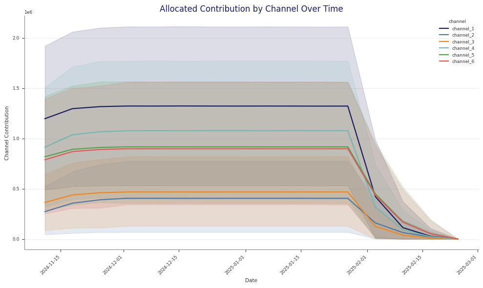
Plot the result

The plotting helpers under mmm.plot are designed to work directly with the response dataset returned by the wrapper.

fig, ax = mmm.plot.budget_allocation(response_samples, original_scale=True)

fig, ax = mmm.plot.allocated_contribution_by_channel_over_time(
    response_samples,
    original_scale=True,
)

Useful options:

• dims={...} to filter a panel slice
• split_by="geo" or another dimension to create separate subplots
• original_scale=True to prefer original-scale contribution variables when they are available

Example optimisation output:

Read the Stage 70 pipeline artefacts

If you run optimisation through python -m abacus.pipeline.runner, Stage 70 writes both the low-level optimiser output and several interpretation files.

The stage also writes plots for allocation, contribution over time, response curves, impact, bounds audit, and ROI or CPA summaries.

These Stage 70 spend figures are reported in total horizon spend units so they can be compared directly to current historical spend over the same reference window. Abacus still converts to the low-level wrapper’s per-period budget contract internally.

Practical checks

Before you use an optimised plan, check:

• result.success and result.message
• whether the allocation matches your intended budget units
• whether budget_bounds_audit.csv or your own checks show any bound issues
• how much of the gain comes from reallocation versus carryover assumptions
• whether the point lies on a sensible part of the response curve, not just on the edge of a bound

For multi-plan comparison in total horizon units, use Scenario Planning.

Scenario Planner

The detailed planner documentation now lives in Scenario Planning.

Use that section for:

• planner concepts and workflow
• scenario specification classes
• Python API examples for abacus.scenarios.ScenarioPlanner
• comparison output tables
• retained YAML recipes through the abacus.scenarios CLI

The planner is a higher-level surface than Budget Optimisation:

• PanelBudgetOptimizerWrapper uses per-period spend units
• abacus.scenarios.ScenarioPlanner uses total horizon spend units

Start here:

• Scenario Planning
• Overview and Workflow
• Python API