ABACUS is a Bayesian MMM library built on PyMC and PyTensor.
The public PanelMMM API includes released named presets for one aggregate
time series, one-unit fixed effects (FE), and one-unit correlated random effects
(CRE). Start with Choose an Estimator
before preparing a panel model. The random-effects (re) preset remains
release-gated.
Start with a task
These Markdown pages describe the Abacus checkout they accompany. Open the
section indexes directly in your repository viewer or editor; keep the
library and documentation at the same revision.
The YAML builder returns a built model for
subsequent fitting and analysis. The runner
executes a staged workflow and writes artefacts to disk. Their configuration
surfaces differ; use the tutorial for the route you intend to run.
the repo-managed development environment from environment.yml
an editable install, so local code changes are picked up immediately
Minimal pip install from source
If you do not want the full Conda environment, you can still install Abacus
directly from the repository root.
Standard install
python3 -m pip install .
Editable install
python3 -m pip install -e .
Use the editable install if you are changing code, configs, or docs locally.
Optional extras
Abacus defines a small set of optional extras in pyproject.toml.
Extra
Install command
Use when you need
lint
python3 -m pip install .[lint]
Ruff, MyPy, and related local linting tools
test
python3 -m pip install .[test]
Pytest and test-only dependencies
planner
python3 -m pip install -e ".[planner]"
Deprecated no-op compatibility marker for old install commands
If you created the environment from environment.yml, most development
dependencies are already present.
The statistical scenario API does not require the planner extra. New
library code should import scenario objects from abacus.scenarios. The
experimental abacus-dashboard application is deprecated. Use the scenario
Python API or CLI; no dashboard installation is required. Legacy app-layer
paths under abacus.scenario_planner remain as advisory compatibility facades.
Abacus does not vendor Dash, Plotly, or Flask dependencies.
For a real end-to-end verification path, use the repo smoke target:
make smoke_mmm
If you are working on the repo itself, the main local verification commands
are:
make testmake verify_local
make verify_package
Runtime defaults for restricted environments
Some local runs need writable cache directories. If you hit PyTensor compiledir
or cache-permission issues, export the same defaults used by the repo
verification scripts:
This page shows the fastest direct path from a pandas dataset to a fitted
PanelMMM.
If you have not prepared your dataset yet, read
Data Preparation first.
Load a dataset
The repository includes bundled demo datasets under data/demo/. The
timeseries bundle is the simplest starting point because it has no extra panel
dimensions.
An existing model graph can only be fitted with the data used to construct it.
This applies to both fit() and approximate_fit(), including models restored
with PanelMMM.load(). Equal copies of the training inputs are accepted;
changed outcomes, predictors, dates or panel units raise ValueError before
inference starts. Use a fresh model instance to fit a different dataset.
Abacus checks the retained training values and coordinates, not Python object
identity. Mutating the original DataFrame or array after construction does not
change the recorded training data. The check also rejects fitting after an
in-place update of the graph’s training data. Posterior prediction clones the
PanelMMM graph by default; keep that default if you intend to fit it again.
Building explicitly and then fitting identical data preserves additions to the
graph, including calibration terms and extra deterministics. Abacus does not
silently rebuild the graph when fitting inputs change.
Supply the real target when constructing a graph for prior predictive checks
that you intend to fit later:
Omitting y during prior construction creates a graph with zero targets. A
later fit with different target values is rejected; construct a fresh instance
for that fit.
This guard does not retrospectively validate saved results. If an earlier fit
reused a graph with changed inputs, rerun it from a fresh instance.
Read Model Fitting for fitting, save/load, and
predictive-check workflows in more detail.
Quickstart: YAML Builder
Use the YAML builder to create an in-memory PanelMMM from a model
specification. It builds the PyMC graph; you then fit and predict in Python.
For staged outputs and manifests, use the
Pipeline Runner.
Complete Installation first. The example below uses small
synthetic data and short chains to check execution. It does not establish
convergence, parameter recovery or a suitable model for real data.
Create a builder configuration
Work in a new scratch directory, such as sandbox/yaml-quickstart/ within your
checkout. Save this as model.yml in that directory:
This configuration accepts X and y from Python. The bundled
data/demo/timeseries/config.yml is a runner configuration: it also
contains diagnostics, validation, prior_sensitivity and ai_advisor.
The public builder rejects those runner-only blocks. Use the runner for that
file; do not pass it directly to build_mmm_from_yaml(...).
Build from synthetic data
Run these Python blocks in order from the directory containing model.yml:
With this configuration, the returned dataset has 24 dates and 100 combined
posterior samples (two chains of 50 draws). Sampling warnings and divergences can occur
with such short chains. Do not interpret these smoke-run estimates. Before
interpreting a real model, choose adequate sampling settings and assess
Diagnostics.
Override configuration from Python
model_kwargs takes precedence over the translated YAML constructor arguments.
For sampler_config, provide the complete mapping you want to use: it replaces
the YAML sampler mapping at this boundary.
This second fit only checks the override path. It is not a sensitivity or
convergence assessment.
Load your own data
Pattern
What you provide
In-memory data
Both X and y, as above
Combined CSV
data.dataset_path; the file must contain the target column
Separate CSVs
data.x_path and data.y_path
Configured relative paths resolve from the YAML file’s directory. The builder
normalises the configured date column. To fit after loading a CSV, load and
split that data in Python too, then pass matching X and y to fit(...).
See Input Data Requirements
for index, missing-data and panel rules.
Optional builder blocks
Key
Purpose
estimator
Select a named estimator preset
dimensions
Legacy panel-dimension configuration; do not combine with estimator
scaling
Target and channel scaling rules
effects
Additive effects attached before graph construction
priors
Model-level prior overrides
fit
Sampler defaults
holidays
Holiday/event configuration
original_scale_vars
Original-scale deterministic variables added after build
inference_data
Attach saved inference data
calibration
Calibration steps after build, subject to estimator support
optimization
Optimisation settings accepted by the shared schema; the builder does not run optimisation
Use the pipeline runner when you want a full staged run instead of only an
in-memory model fit.
The runner writes:
a run manifest
copied and resolved config files
fitted model artefacts
posterior predictive assessment outputs
decomposition, diagnostics, and response-curve artefacts
Full bundled demo
From the repository root, run the complete demo with:
python3 runme.py --demo timeseries
Other bundled demos are:
timeseries_controls
geo_fe
geo_cre
geo_panel
geo_brand_panel
timeseries and timeseries_controls use the released time_series estimator
preset. geo_fe and geo_cre use the released one-unit FE and CRE presets.
geo_panel and geo_brand_panel use the advanced dimensions.panel surface;
they are not named RE, FE, or CRE estimators. The named RE preset remains
release-gated. See the demo catalogue for the exact
semantics and release status of each recipe.
List them explicitly with:
python3 runme.py --list-demos
runme.py is a convenience wrapper around the structured pipeline. It resolves
the demo config under data/demo/<demo_name>/config.yml and runs the pipeline
for you.
Read Choose an Estimator
before treating either recipe as the basis for a real model.
The timeseries demo requests four chains with 2,000 tuning and 3,000 retained
draws per chain for Stage 20. Its enabled validation stage separately requests
four chains with 2,000 tuning and 2,000 retained draws per chain. Explicit
validation.sampler settings override main-fit CLI settings for that refit.
make smoke_mmm launches this full demo without reducing either budget.
Bounded software smoke
Use this synthetic example to check execution with a small, explicit budget.
Run the following from the repository root in the installed Abacus environment.
It creates a separate scratch configuration and dataset, leaving the bundled
demos unchanged. Repeating the setup overwrites these two scratch inputs; each
pipeline execution creates a new run directory.
Stage 20 uses two chains, each with 20 tuning and 20 retained draws, on one
core. Stage 35 performs no fit: run_manifest.json must record validation as
skipped, and no holdout scoring artefacts are expected. Prior sensitivity,
both AI stages and optimisation are also skipped because their configuration
blocks are absent. The run should complete through Stage 80’s evidence
inventory. The resolved main-fit settings are in
00_run_metadata/config.resolved.yaml.
These small sampling budgets check software execution only. Warnings or
retained divergences can occur; do not interpret these fitted estimates.
To exercise holdout scoring, prepare a separate config with explicit budgets
for both fits and follow Blocked Holdout Validation.
A skipped validation stage is not evidence of predictive performance.
Run the pipeline from Python
The direct Python API below runs the bundled geo-panel model. It is separate
from the bounded synthetic smoke above. Check the selected YAML’s validation
budget before running it:
The CLI prints the final run directory and manifest when the pipeline
completes. When the run manifest records them, it also prints paths to the
estimator summary, diagnostics summary, and interpretation report. These paths
are relative to the run directory.
Pipeline completion means that the configured stages finished. It does not
mean that the fitted model passed its diagnostic gates or is suitable for
interpretation. Review the listed diagnostic and interpretation artefacts
before using model outputs.
Override data paths
Use one of these patterns:
Pattern
Arguments
Combined dataset override
dataset_path= in Python or --dataset-path in the CLI
Separate feature and target files
x_path= and y_path= in Python or --x-path and --y-path in the CLI
Target column override
target_column= in Python or --target-column in the CLI
Configured relative paths are resolved relative to the YAML config directory.
If you want Stage 50 to use different warn/fail cutoffs, add a runner-only
diagnostics.thresholds block to the YAML. See
YAML Configuration.
What you get back
run_pipeline(...) returns a PipelineRunResult with:
run_dir
manifest_path
The runner creates all stage directories up front, including those for skipped
stages. Use the manifest to distinguish completed, skipped and failed work.
See the canonical stage sequence
and artefact locations, including
Stage 80’s evidence inventory.
Named estimator runs also record their resolved contract in
00_run_metadata/estimator_summary.txt and
00_run_metadata/estimator_manifest.yaml. FE writes its transformed
within-design screen under 10_pre_diagnostics. CRE writes structural and
reference summary-basis screens under 10_pre_diagnostics, a bounded post-fit
screen under 20_model_fit, and separate CRE-adjustment decomposition evidence
under 40_decomposition.
60_response_curves now includes three complementary curve families:
saturation-only transformation artefacts
forward-pass direct contribution artefacts built from scaled observed history
This section explains how to prepare X and y for PanelMMM.
It covers the required columns, how panel rows are organised when you use
dims or a named FE or CRE estimator, and how Abacus scales channels and the
target before fitting.
Pages
Input Data Requirements — Required X and y
inputs, column roles, alignment rules, and common input errors.
Panel Data Layout — How to structure rows for named
FE and CRE panels, no panel dims, one dim such as geo, or multiple dims
such as geo and brand.
Scaling and Preprocessing — What Abacus
scales automatically, how Scaling works, and what to preprocess yourself.
y as a row-aligned pandas.Series, or a one-dimensional NumPy
array of the same length as X
X must contain the date column, all media columns, and any configured
control_columns or dims columns. y carries only the target values.
Role
Where it must be present
Required
Notes
date_column
X
Yes
Normalise to datetimes or parseable date strings.
channel_columns
X
Yes
Every listed channel column must exist in X.
target_column
y
Yes
Abacus uses target_column as the internal name.
control_columns
X
No
If configured, every listed control column must exist in X.
dims
X
No
One column per configured panel dimension, such as geo or brand.
X and y
When you call fit(X, y) or build_model(X, y):
Keep the target out of X.
Keep X and y row-aligned.
If both are pandas objects, keep the same index on both. The shared
regression builder checks index equality before fitting.
If you pass y as a NumPy array, its length must match len(X).
For panel models, each date_column + dims combination must appear
exactly once. Duplicate rows are rejected.
Abacus uses target_column as the target name throughout the panel reshape.
A Series name is normalised internally without changing the caller’s Series.
Date column
date_column is required in X.
Abacus expects calendar dates, not integer date codes. In practice:
Use datetime64[ns] where possible.
Parse string dates with pd.to_datetime(...) before fitting when you use the
Python API.
Do not rely on numeric date values such as 0, 1, 2. Pandas can interpret
them as offsets from the Unix epoch, which is usually not what you want.
The YAML builder normalises X[date_column] with pd.to_datetime(...) after
loading the dataset. Direct Python use does not add an equivalent preprocessing
step for you.
Channel columns
channel_columns is a required constructor argument and must be a non-empty
list.
Each listed channel:
must be present in X
must be fully observed for every row you pass into fit or posterior
prediction; Abacus does not silently convert missing channel values to zero
should represent the raw media variable that you want the adstock and
saturation transformations to consume
Target column
target_column names the dependent variable. It defaults to "y", but you can
set a different name such as "sales" or "conversions".
For direct Python use:
pass the target as y
keep the target fully observed; missing target values are rejected rather
than zero-filled
For combined-file YAML or pipeline flows:
keep the target column in the source dataset
Abacus splits it out of the combined dataset before fitting
Control columns
control_columns is optional.
If you configure it, every listed control column must be present in X.
Controls stay in the design matrix as separate regressors; they are not part of
y.
Like channels, configured controls must be fully observed for every row passed
into fit or posterior prediction.
One tabular file containing both predictors and the target column
Pipeline runner with dataset_path
Same as above
Pipeline runner with x_path and y_path
Separate feature and target files; the runner extracts target_column from the target file
Abacus also has an internal alignment helper that can work with a MultiIndex
target Series indexed by [date_column, *dims], but that is mainly used in
fit-data rebuild and load flows. For normal fitting, keep y row-aligned with
X.
For PanelMMM.build_model(X, y) and fitting, a one-dimensional NumPy target
is positional: its length must equal len(X), and values follow X’s row order
regardless of whether X uses a RangeIndex, an offset index or a DatetimeIndex.
A pandas Series target must have exactly the same row index as X. Prepared
observations and retained fitting provenance use the same alignment rule.
Common pitfalls
Missing date_column, channel, control, or dimension columns in X
Passing pandas X and y with different indexes
Passing a NumPy y with a different length from X
Passing duplicate panel rows or incomplete panel slices for a given date
Passing missing observed channel, control, or target values and expecting
Abacus to treat them as structural zeroes
Expecting the YAML builder or pipeline to find a target column that is not
present in the combined dataset
Leaving date values as numeric codes instead of normalising them first
Panel Data Layout
This page explains how PanelMMM expects panel rows to be organised in X.
For the column-level contract, see
Input Data Requirements.
What “panel” means in Abacus
In Abacus, a panel dataset repeats the same time axis across one or more
categorical dimensions in dims.
The released FE and CRE presets are more specific one-unit panel contracts.
They declare estimator.type: fe or estimator.type: cre and
estimator.unit: <column> instead of dimensions.panel. Both require the same
date set for every unit, so their released surfaces use a balanced unit-date
panel. See Choose an Estimator,
Fixed-effects Estimator,
and Correlated-random-effects Estimator.
Each row represents:
one date_column value
one combination of dims values, if any
one set of channel and optional control values for that slice
With no extra panel dims, each date appears once. With dims=("geo",), each
date appears once per geo. With dims=("geo", "brand"), each date appears
once per geo + brand combination.
How dims work
Pass panel dimensions when you construct the model:
Abacus converts the pandas inputs into xarray datasets before building the
PyMC model.
Input role
Internal variable
xarray dims
X[channel_columns]
_channel
(date, *dims, channel)
X[control_columns]
_control
(date, *dims, control)
y
_target
(date, *dims)
The channel and control dimensions come from the configured column names,
not from row values.
Rectangularity, duplicates, and missing rows
Abacus builds xarray coordinates from the unique values it sees in:
date_column
each configured dimension column
the configured channel or control names
That has three practical consequences:
Keep the panel rectangular. Provide one row for every expected
date_column + dims combination.
Use explicit zeroes for structural no-spend or no-activity rows.
Keep declared channel, control, and target values observed within those rows.
Abacus rejects missing metric cells instead of silently converting them to
zeroes.
Do not use missing rows to mean “unknown”. Abacus validates panel shape
before reshape and raises an error if panel cells are missing.
Abacus also requires each date_column + dims combination to appear exactly
once. It does not aggregate duplicates for you. If you have duplicate rows,
deduplicate or aggregate them before fitting or posterior prediction.
Sorting and uniqueness
Sort your data before fitting:
first by date_column
then by each entry in dims
Abacus keeps dates in the order they appear in X, and time-varying features
infer time resolution from adjacent rows. A sorted dataset makes the time axis
deterministic and easier to reason about.
Also make sure that each date_column + dims combination appears once in the
prepared table, and that every expected panel slice is present for every date.
DataFrame versus MultiIndex handling
For normal fitting:
use a regular DataFrame for X
keep date_column and any dims as columns in that DataFrame
use a row-aligned Series for y
Abacus does have internal helpers that can align a MultiIndex target Series
indexed by [date_column, *dims], but that is not the main user-facing data
preparation pattern for fit().
Practical checklist
One row per date_column + dims combination
No duplicate rows for the same panel cell
Same set of dates for every panel slice
Explicit zeroes for true zero activity
No missing observed channel, control, or target values
Sorted rows before fitting
For FE or CRE, exactly one declared unit column with at least two units and
two dates
For FE or CRE, non-zero within-unit temporal variation in the target and
each estimable transformed predictor
For CRE, enough units to estimate the active centred summaries while
retaining at least two between-unit residual degrees of freedom
Abacus scales channels and the target automatically before it builds the PyMC
graph for PanelMMM. This page explains what is scaled, how the Scaling
configuration works, and what you still need to preprocess yourself.
What Abacus scales automatically
Abacus computes scales from the reshaped xarray dataset immediately before model
construction.
Variable role
Automatic scaling
Notes
Target (y)
Yes
Divided by target_scale before the likelihood is built.
Channels (channel_columns)
Yes
Divided by channel_scale before adstock and saturation.
Controls (control_columns)
No
Controls enter the model on their original scale.
Date and dims columns
No
These define coordinates, not modelled numeric inputs.
Abacus stores the resulting scalers in the model as xarray data:
The YAML builder supports the same workflow through original_scale_vars:
original_scale_vars:- channel_contribution- y
original_scale_vars adds extra original-scale deterministic variables. It
does not change how the model is fit.
What Abacus does not preprocess for you
Abacus does not automatically:
scale controls
impute missing data in a domain-aware way
reinterpret missing observed channel, control, or target values as zeroes
sort the dataset for you
repair non-rectangular panel layouts
tolerate duplicate panel rows or incomplete panel slices
coerce Python-API dates to datetimes before fitting
Practical preprocessing advice
Before fitting:
normalise date_column with pd.to_datetime(...)
sort by date_column and then by dims
make panel gaps explicit instead of leaving missing rows
ensure every date_column + dims panel cell appears exactly once
impute missing observed channel, control, and target values before fitting or
posterior prediction instead of relying on implicit zero-fill
decide whether controls should be centred, standardised, log-transformed, or
otherwise prepared before they go into control_columns
choose scaling dims deliberately instead of relying on the default when you
use panel data
Common pitfalls
Expecting the default scaling to be per-group when it actually pools across
the configured panel dims
Adding date to VariableScaling.dims; Abacus rejects this
Forgetting that controls are left on their original scale
Treating VariableScaling.dims as dimensions to keep rather than dimensions
to reduce across
Assuming original_scale_vars changes fitting scale rather than adding extra
outputs
For the input table shape that scaling operates on, see
Panel Data Layout.
Model Specification
This section explains how PanelMMM is defined: the model structure, media
transforms, priors, panel dimensions, optional time variation, and calibration
hooks.
Pages
Model Overview - The actual PanelMMM mean structure,
scaled-space formulation, and optional components.
Adstock and Saturation - Supported media
transforms, their priors, and the adstock_first composition order.
Priors and Configuration - Default prior keys,
model_config, transform-prior overrides, and directional control priors.
Time-Varying Parameters - How
time_varying_intercept and time_varying_media use SoftPlusHSGP.
Seasonality and Trends - Built-in yearly
seasonality plus custom Fourier, trend, and event effects.
Panel Dimensions - How dims change the shape of the
data and parameters.
Choose an Estimator - Compare the released
time-series, FE, and CRE contracts and choose the identifying variation that
matches the modelling question.
Fixed-effects Estimator - The released
one-unit FE contract, its within-design checks, and its limits.
The released one-unit CRE contract, its transformed summary basis,
estimability checks, and interpretation limits.
Calibration - Lift-test and cost-per-target calibration for
a built model.
Subsections of Model Specification
Model Overview
PanelMMM is an additive Bayesian marketing mix model built in PyMC. This page
describes the model structure that Abacus actually builds.
For input layout, see Data Preparation. For
individual configuration surfaces, see the other pages in this section. Named
FE and CRE presets use specialised likelihoods and restrictions; read
Choose an Estimator before applying this general
component description to them.
Core structure
At fit time, Abacus builds the model mean in scaled target space as:
mu =
  intercept_contribution
  + sum(channel_contribution over channel)
  + sum(control_contribution over control), if control_columns are configured
  + mundlak_contribution, if use_mundlak_cre=True
  + yearly_seasonality_contribution, if yearly_seasonality is enabled
  + any additional mu_effects
The observed target is then attached through the configured likelihood
distribution with mu=mu.
What is scaled and what is not
Before the PyMC graph is built:
channel data is scaled according to Scaling.channel
the target is scaled according to Scaling.target
controls are not scaled automatically
That means media and target priors operate on the model scale, not directly on
the original business units. For the scaling surface, see
Scaling and Preprocessing.
Model components
Component
Built when
Shape
intercept_contribution
Always
effectively ("date", *dims) in the model mean
channel_contribution
Always
("date", *dims, "channel")
control_contribution
control_columns is set
("date", *dims, "control")
mundlak_contribution
use_mundlak_cre=True
dims
yearly_seasonality_contribution
yearly_seasonality is set
("date", *dims)
Additional additive effects
You add entries to mu_effects
("date", *dims)
Abacus also adds total_media_contribution_original_scale automatically as a
deterministic on the original target scale.
Media path
Each channel column goes through the configured media transform path:
scale channel input
apply adstock and saturation through forward_pass(...)
optionally apply a time-varying media multiplier
contribute the result through channel_contribution
Use controls for non-media regressors such as price, macro indicators, or
competitor measures. Controls are configured with control_columns and use
gamma_control priors from model_config.
Panel dimensions
dims adds extra indexing axes such as geo, brand, or market.
With dims=("geo",), the model is indexed over date and geo. With
dims=("geo", "brand"), it is indexed over date, geo, and brand.
Abacus does not automatically add hierarchical pooling just because dims is
set. By default, parameters are indexed over the configured panel coordinates.
If you want hierarchical shrinkage across those coordinates, encode it in the
priors you pass to transforms or model_config.
This table describes the ordinary PanelMMM component surface. The released
FE and CRE presets deliberately reject several optional components and
downstream operations. Their estimator pages are authoritative for those
boundaries.
What target_type changes
target_type is semantic metadata, not a different likelihood family.
It affects downstream reporting such as the default efficiency metric label:
"revenue" -> ROAS
"conversion" -> CPA
It does not change the fitted functional form on its own.
Read Choose an Estimator before choosing an
aggregate time-series, FE, or CRE contract.
Adstock and Saturation
PanelMMM requires one adstock transform and one saturation transform. Abacus
applies them inside the model graph rather than as a fixed preprocessing step.
Transform priors also appear in model_config under prefixed variable names.
For example:
adstock_alpha
adstock_lam
adstock_k
saturation_lam
saturation_beta
That means you can override transform priors centrally through the top-level priors
if you prefer. See Priors and Configuration.
Choose the composition order
adstock_first is part of the model specification, not a plotting choice.
The current public YAML schema does not expose adstock_first; it uses the
library default. If you need to change the composition order, use the Python
API.
Use adstock_first=True when you want the model to interpret carryover before
diminishing returns. Use False when you want each period’s spend to saturate
before the carryover step.
The code path is explicit:
True -> saturation(adstock(x))
False -> adstock(saturation(x))
Common pitfalls
Forgetting that l_max is required for adstock classes
Assuming dims automatically change transform priors even when you have
already set explicit incompatible dims on the transform
Using adstock_first=False without a substantive reason
Treating transform priors as if they were on original business units rather
than the model scale
The builder appends these effects before calling build_model(...).
Choosing between built-in and custom seasonality
Use yearly_seasonality when you need a compact built-in annual effect.
Use FourierEffect when you need:
weekly seasonality
monthly seasonality
multiple seasonal effects together
custom Fourier prefixes or priors
Common pitfalls
Adding effects after the model has already been built
Using event effect dims that do not include the required prefix
Treating yearly_seasonality and a custom yearly Fourier effect as if they
were separate concepts when they are both additive seasonal terms
Next steps
Read Time-Varying Parameters if you want trend
or media behaviour to vary smoothly over time.
Read Calibration if you want to constrain the specification
with external measurements.
Priors and Configuration
Abacus uses model_config to control priors on the underlying PyMC variables.
Transform priors can be configured either on the transform objects themselves or
through their prefixed variable names in model_config.
Abacus parses these mappings into runtime Prior or HSGPKwargs objects.
Transform priors and prefixed names
Transform parameters appear in the model under prefixed variable names.
Examples:
adstock alpha -> adstock_alpha
saturation lam -> saturation_lam
saturation beta -> saturation_beta
So you can override transform priors in either of these ways:
pass priors={...} to the transform object
override the prefixed variable in model_config
Use one style consistently within a project if you want the configuration to be
easy to read.
Directional control priors
Controls are the right place for exogenous drivers whose effect may be
negative, such as competitor spend, competitor price pressure, or supply-side
disruptions. By default, control coefficients remain unrestricted.
The current public YAML schema does not expose control_impacts or
control_sign_policy. If you need directional control settings today, use the
Python API for that part of the specification.
Constraints for directional controls
When control_impacts is configured, Abacus expects:
gamma_control and gamma_control_mundlak to be Normal or
TruncatedNormal
scalar numeric mu and sigma values for those priors
the prior dims to include "control"
If you violate those assumptions, model build fails with a validation error.
Time-varying configuration keys
When you enable a boolean time-varying effect, Abacus uses these model_config
keys:
intercept_tvp_config
media_tvp_config
Those keys can be:
an HSGPKwargs instance
a dict with HSGPKwargs fields
a dict in SoftPlusHSGP.parameterize_from_data(...) style, such as
{"ls_lower": 1, "ls_upper": 10}
dims tells PanelMMM which extra categorical axes exist alongside date.
With no extra dims, the model is indexed by:
date
channel
optionally control
With dims=("geo",), the model is indexed by:
date
geo
channel
optionally control
With dims=("geo", "brand"), it is indexed by:
date
geo
brand
channel
optionally control
What changes inside the model
Setting dims changes the coordinates and parameter shapes used in the PyMC
graph.
Quantity
No extra dims
dims=("geo",)
channel_data
("date", "channel")
("date", "geo", "channel")
target_data
("date",)
("date", "geo")
channel_contribution
("date", "channel")
("date", "geo", "channel")
control_contribution
("date", "control")
("date", "geo", "control")
intercept prior dims by default
()
("geo",)
Reserved names
Do not use these names in dims:
date
channel
control
fourier_mode
Abacus rejects them because they are reserved for internal coordinates.
dims does not imply automatic pooling
This is the most important modelling point.
By default, dims gives you parameters indexed by the panel coordinates, but
not automatic hierarchical shrinkage across those coordinates.
For example:
the default intercept prior is Normal(..., dims=dims)
transform priors default to (*dims, "channel")
control coefficients default to (*dims, "control")
Those defaults create per-slice parameters. If you want hierarchical pooling
across geo, brand, or another dimension, you need to encode that in the
priors you supply.
You can do the same for transform priors and additive effects.
Legacy Mundlak adjustment and panel dimensions
use_mundlak_cre=True only makes sense when you have at least one panel dim.
Abacus enforces that. This low-level surface is not the named CRE estimator
preset, and its coefficients do not by themselves identify confounding or
establish causal effects.
When enabled, Abacus builds extra correlated-random-effects terms from training
period means:
channel_mundlak_contribution
control_mundlak_contribution
mundlak_contribution
These terms live on the panel coordinates defined by dims.
Custom HSGP dims
If you use a custom SoftPlusHSGP for time-varying effects, its dims must be
compatible with the panel structure.
Examples:
no extra dims: ("date",) or ("date", "channel") for media
dims=("geo",): ("date", "geo") or ("date", "geo", "channel") for media
Calibration lets you add external evidence to a built PanelMMM.
Both calibration methods are unavailable for the named FE, CRE and
release-gated RE presets; they raise EstimatorOperationError. Check
Choose an Estimator before
preparing calibration data. A built graph alone does not establish support.
Abacus currently supports two retained calibration paths:
lift-test measurements through add_lift_test_measurements(...)
cost-per-target calibration through add_cost_per_target_calibration(...)
General rule
Both calibration methods operate on a built model, not a bare constructor.
only the supported calibration methods above are available in YAML
dist is not supported in YAML yet for add_lift_test_measurements
other calibration actions should be applied through the Python API until they
have explicit YAML support
Choose the right calibration path
Use lift tests when you have measured incremental response data for a specific
spend change.
Use cost-per-target calibration when you want the fitted channel contribution to
stay consistent with observed cost efficiency.
For a supported estimator, you can use either or both after building the model.
Common pitfalls
Adding calibration before build_model(...)
Forgetting to add channel_contribution_original_scale before
cost-per-target calibration
Omitting required dims columns from calibration data
Assuming YAML supports every Python calibration argument; dist does not
currently round-trip through YAML
Next steps
Read Model Fitting for the fit workflow once the
model has been fully specified.
Read Save and Load if you plan to keep
calibrated models on disk.
Correlated-random-effects Estimator
The released cre preset fits a one-unit correlated-random-effects (CRE)
marketing-mix model. It combines shared media and control slopes with a
Gaussian random unit intercept and an explicit adjustment for association
between persistent unit differences and the declared predictors.
Released contract
estimator:type:creunit:geo
The v1 surface has these deliberate limits:
Component
Released CRE behaviour
Unit dimensions
Exactly one categorical unit column
Unit effects
Gaussian random intercept, integrated out exactly
Media and control slopes
Shared across units
Adstock and saturation
Shared geometric adstock followed by logistic saturation
CRE media summaries
Centred unit means of the transformed exposure basis
CRE control summaries
Standardised centred unit means of eligible time-varying controls
Residual scale
Shared across units
Common time effects and seasonality
Not supported
Custom additive effects and holidays
Not supported
Historical and manual scenarios
Supported for the complete fitted-unit panel; fitted CRE summaries remain frozen
Calibration and fixed-budget optimisation
Not supported
Use the bundled starting point at data/demo/geo_cre/config.yml.
Run it from the repository root:
python3 runme.py --demo geo_cre
Statistical meaning
For unit i and date t, CRE augments the shared-slope level equation with
unit summaries of the declared regressors. The media summaries are computed
from the fitted adstock-and-saturation exposure basis. They are not raw-spend
means. Eligible control summaries are standardised unit means.
The residual unit intercept is integrated out. The likelihood therefore uses
one exact Gaussian covariance block per unit. Pointwise log likelihood is
unit-block marginal evidence, not an observation-level or future-date score.
The adjustment relaxes the naive random-effects mean-independence restriction
only with respect to the declared summary basis. It does not establish causal
identification or address omitted time-varying confounding, measurement error,
reverse causality, or response-function misspecification.
Data and estimability requirements
The dataset must be a balanced unit-date Cartesian product with one row per
unit and date. It must contain enough units to estimate the active centred
media and control summaries while retaining at least two residual between-unit
degrees of freedom.
Abacus rejects:
non-finite predictors or targets;
media with no within-unit temporal variation;
an exactly rank-deficient transformed between-summary design; and
insufficient between-unit residual degrees of freedom.
It warns about low transformed within-unit variation, high variance inflation
factors, and a high condition number. These thresholds are configurable under
estimator.estimability. A pass means that the implemented screen found no
declared defect. It is not proof of global, posterior-wide, or causal
identification.
After fitting, inspect posterior convergence, effective sample size, sampler
pathologies, prior sensitivity, the post-fit summary-basis diagnostics, and
predictive checks. A CRE coefficient interval containing zero does not prove
that a simpler random-effects model is adequate.
Pipeline evidence
A structured CRE run records:
the resolved estimator contract in
00_run_metadata/estimator_summary.txt and
00_run_metadata/estimator_manifest.yaml;
the raw structural screen in
10_pre_diagnostics/cre_structural_estimability.json;
the transformed reference-basis screen in
10_pre_diagnostics/cre_reference_estimability.json and
10_pre_diagnostics/cre_reference_estimability_features.csv;
the bounded posterior-draw screen in
20_model_fit/cre_postfit_estimability.json; and
the CRE adjustment and reconciliation outputs under 40_decomposition.
The run manifest is the machine-readable index of these files. A completed
pipeline only means that every required stage ran. Review the diagnostic status
before interpreting the posterior.
Prediction and persistence
Prediction is conditional on the fitted unit history. Every prediction request
must supply all fitted units. Row order may vary, but unseen units and
fitted-unit subsets are rejected. Save and load preserve the fitted CRE summary
state and validate its unit coordinates before prediction.
Historical and manual scenarios use the same fitted-unit restriction. Manual
spend changes the nonlinear media-response path, but Abacus does not recompute
the fitted training-period Mundlak media or control summaries. This preserves
the fitted CRE adjustment rather than redefining confounding context from the
planned spend. Scenario outputs are posterior media-contribution estimates,
not total-outcome forecasts or causal effects.
Use the YAML and Python examples under data/demo/geo_cre/. Fixed-budget
optimisation remains outside the released CRE scenario contract.
Evidence boundary
The release verifies the declared graph, configuration restrictions,
estimability evidence, fitted-unit prediction contract and persistence path.
It does not promise a fixed point-estimate accuracy, causal validity, or general
robustness for arbitrary data. Treat each fitted model as a separate statistical
assessment.
For a direct comparison with FE and the aggregate time-series preset, see
Choose an Estimator.
Choose an Estimator
PanelMMM provides three released named estimator presets:
time_series for one aggregate time series
fe for a one-unit fixed-effects panel
cre for a one-unit correlated-random-effects panel
The re declaration is typed but release-gated. It is not a runnable
estimator.
Release support matrix
Preset
Status in 3.1.1
Data contract
Identifying variation
Important operation boundary
time_series
Released
One aggregate observation per date
Aggregate temporal variation
Uses the supported ordinary PanelMMM workflow
fe
Released
One balanced unit-date panel
Within-unit temporal variation
Prediction and historical/manual scenarios require all fitted units; calibration and fixed-budget optimisation are unavailable
cre
Released
One balanced unit-date panel
Within-unit variation conditional on the declared transformed between-unit summary adjustment
Prediction and historical/manual scenarios require all fitted units and frozen fitted CRE summaries; calibration and fixed-budget optimisation are unavailable
re
Gated; not released
Declaration only
Not applicable until release
Graph construction fails closed with EstimatorReleaseGateError
The support status is a software release boundary, not evidence that a preset
is appropriate for a particular dataset or causal question.
Compare the released presets
Question
time_series
fe
cre
Data structure
One observation per date
Balanced unit-date panel
Balanced unit-date panel
Unit effects
Not applicable
Absorbed unit intercepts
Gaussian random unit intercept
Identifying variation for shared slopes
Aggregate temporal variation
Within-unit temporal variation
Within-unit temporal variation, conditional on the declared between-unit summary adjustment
Media slopes
Shared
Shared across units
Shared across units
Adstock and saturation
Shared
Shared across units
Shared across units
Persistent unit differences
Not represented
Removed from the slope likelihood
Modelled through the random intercept and declared CRE summaries
Common categorical time effects
Not an estimator option
Not supported
Not supported
Calibration
Available through the ordinary PanelMMM surface
Not supported
Not supported
Historical and manual scenarios
Supported
Supported for all fitted units
Supported for all fitted units with frozen fitted CRE summaries
Fixed-budget optimisation
Supported
Not supported
Not supported
All three presets combine likelihood information with the declared priors.
None of them turns observational marketing data into a causal design.
Use the time-series preset
Use time_series when the modelling unit is one aggregate market, brand, or
business series and each date occurs once.
estimator:type:time_series
Do not use it to disguise panel observations as independent aggregate rows.
Aggregate the data deliberately or use a panel estimator.
Use FE
Use fe when the target question concerns changes within units over time and
you want time-invariant unit characteristics removed from the shared-slope
likelihood.
estimator:type:feunit:geo
FE is appropriate only when the transformed media and controls have enough
within-unit temporal variation. It cannot estimate coefficients for predictors
that are constant within every unit. It also does not remove time-varying
confounding or common shocks.
Use cre when persistent unit differences may be associated with the declared
predictors and you need an explicit within-between panel specification.
estimator:type:creunit:geo
CRE augments the shared-slope random-intercept model with centred unit summaries.
Media summaries use the fitted adstock-and-saturation exposure basis rather
than raw-spend means. The adjustment is limited to the declared basis. It does
not correct arbitrary omitted confounding.
CRE needs both usable within-unit media variation and enough independent
between-unit information for its active summaries. Prediction is limited to
the complete set of fitted units.
The presets answer different statistical questions. Do not select one only
because it has the best in-sample fit, lowest information criterion, or the
most favourable media coefficient.
Before fitting:
State the unit and time structure of the business question.
State which persistent and time-varying confounding paths remain plausible.
Check whether the proposed identifying variation exists after media
transformation.
Choose the estimator contract and priors before inspecting the preferred
result.
After fitting, inspect the estimator-specific estimability evidence, MCMC
diagnostics, posterior predictive checks, prior sensitivity, and any
predeclared holdout evidence supported by that estimator. A passed screen means
that Abacus did not detect the specified defect. It is not proof of causal or
global identification.
The demo sampling settings are evidence-oriented and may take time. Command-line
overrides can reduce the budget for an installation or workflow check. Do not
interpret a reduced run as final statistical evidence.
Fixed-effects Estimator
The released fe preset fits a one-unit fixed-effects marketing-mix model.
It absorbs a separate intercept for each unit and identifies shared media and
control effects from temporal changes within each unit.
For units i and dates t, the level formulation is:
Abacus fits the equivalent exact within-unit orthonormal-contrast likelihood.
The unit intercepts alpha_i are not regularised parameters in the graph.
Consequently, persistent differences between units do not identify the shared
media coefficients.
Released contract
estimator:type:feunit:geo
The released surface has these deliberate limits:
Component
Released FE behaviour
Unit dimensions
Exactly one categorical unit column
Unit effects
Absorbed fixed intercepts
Media and control slopes
Shared across units
Adstock and saturation parameters
Shared across units
Residual scale
Shared across units
Common time effects
Not supported
Annual seasonality and custom additive effects
Not supported
Time-varying intercepts or media
Not supported
Budget optimisation and calibration
Not supported
Use the bundled starting point at
data/demo/geo_fe/config.yml. It contains only settings supported by this
contract.
Run it from the repository root:
python3 runme.py --demo geo_fe
Data requirements
The dataset must be balanced on the declared unit and date columns: every unit
must have the same dates, and each unit-date pair must occur once. It must have
at least two units and two dates.
Each channel and control must vary within at least one fitted unit. A predictor
that is constant within every unit cannot be estimated by FE and causes a
pre-fit error. The target must also have non-zero within-unit variation.
This is not the same as adding geo controls to a pooled model. FE discards
between-geo level variation from the likelihood for the shared slope
coefficients.
Estimability screen
Before the main graph is created, Abacus evaluates media after the configured
adstock and saturation transforms at a fixed-seed PyMC initial point. It saves:
The zero-variation and rank checks remain errors. Do not suppress a warning by
changing a threshold without recording why the underlying design remains fit
for purpose.
The screen is a reference-design diagnostic. It cannot prove identification
for every posterior draw because adstock and saturation parameters are
estimated. A pass is necessary for the released graph, not sufficient evidence
for a causal or decision claim.
Interpretation
For a media channel to be identified, it needs meaningful within-unit temporal
variation after the configured transforms. National media that is identical in
every geography can still vary over time, but it can be difficult to separate
from common shocks. The initial FE contract does not add time fixed effects, so
it does not claim to solve that problem.
FE removes time-invariant unit characteristics. It does not solve time-varying
endogeneity, anticipation, simultaneous promotions, or measurement error. Use
the preflight report, posterior diagnostics, predictive checks, prior
sensitivity, and an explicit causal design before making attribution or budget
decisions.
What comes next
RE and CRE are separate estimator contracts. CRE is released under its own
transformed-summary and prediction boundary; RE remains unavailable.
fit() returns an arviz.InferenceData object and also stores it on
mmm.idata.
What fit() does
When you call fit(X, y), Abacus:
checks that pandas X and y use the same index, if both are pandas
objects
builds the PyMC graph automatically if it has not been built already
merges sampler settings from the model’s sampler_config and your call-time
kwargs
runs pymc.sample(...)
computes deterministic variables and adds them to the posterior group
stores the training data in an InferenceData.fit_data group
writes model metadata into idata.attrs
That means fitted contribution variables such as channel_contribution,
intercept_contribution, and yearly_seasonality_contribution are available
in mmm.posterior after fitting when they are part of the configured model.
Configure the sampler
You can configure PyMC sampling in two places:
Where
Use it for
Precedence
sampler_config= in PanelMMM(...)
Stable defaults you want to reuse across fits
Lower
fit(..., **kwargs)
Run-specific overrides such as draws, chains, or random_seed
Higher
Abacus merges them so that explicit fit() kwargs win.
mmm=PanelMMM(date_column="date",target_column="revenue",channel_columns=["channel_1","channel_2"],adstock=GeometricAdstock(l_max=4),saturation=LogisticSaturation(),sampler_config={"draws":1000,"tune":1000,"chains":4,"target_accept":0.9,"progressbar":False,},)# Overrides draws from sampler_config, keeps target_acceptidata=mmm.fit(X,y,draws=500,random_seed=42)
Common sampler arguments
These are passed through to pymc.sample(...).
Argument
What it controls
draws
Posterior samples kept after tuning
tune
Warm-up or adaptation iterations
chains
Number of MCMC chains
cores
Number of worker processes used by PyMC
target_accept
HMC or NUTS acceptance target
progressbar
Whether PyMC shows a progress bar
random_seed
Sampling reproducibility
If you do not specify progressbar, Abacus defaults it to True unless your
sampler_config already sets it.
When to build first
For a standard workflow, call fit() directly.
Call build_model(X, y) first only when you need to inspect or modify the
graph before sampling. For example:
If you run prior predictive checks first and then call fit(), Abacus keeps
the existing prior and prior_predictive groups on mmm.idata.
That makes it practical to compare:
prior assumptions
posterior fit
posterior predictive behaviour
within one saved InferenceData object.
Common pitfalls
Skipping prior predictive checks and only noticing implausible priors after a
long fit
Treating prior predictive checks as a substitute for posterior predictive
assessment
Forgetting that sample_prior_predictive(...) returns extracted predictive
draws, while the full prior and prior_predictive groups are stored on
mmm.idata
Next steps
After the prior predictive behaviour looks reasonable, fit the model with
Fitting the Model.
Save and Load
Use save and load when you want to persist a fitted PanelMMM and rebuild it
later without redefining the whole model configuration in code.
save() writes the model’s InferenceData to NetCDF. load() reads that file,
recreates the PanelMMM configuration from stored metadata, restores
loaded.idata, and rebuilds the PyMC graph from the saved training data.
What Abacus stores
Abacus relies on more than the posterior draws for a full round trip.
Stored item
Why it matters
posterior and other InferenceData groups
Preserve sampled results
fit_data
Rebuild the model graph with the original training data
idata.attrs
Reconstruct PanelMMM init kwargs and validate compatibility
The stored attrs include both the shared model metadata and PanelMMM-specific
configuration such as:
date_column
channel_columns
target_column
target_type
dims
control_columns
control_impacts
adstock and saturation
adstock_first
yearly_seasonality
time_varying_intercept and time_varying_media
scaling
model_config
sampler_config
serialised mu_effects
save() behaviour
save(fname, **kwargs) is a thin wrapper over self.idata.to_netcdf(...).
Important constraints:
the model must already be fitted
self.idata must contain a posterior group
any extra kwargs are passed directly to InferenceData.to_netcdf(...)
If you call save() before fitting, Abacus raises:
RuntimeError: The model hasn't been fit yet, call .fit() first
load() and compatibility checks
By default, PanelMMM.load(...) validates that the saved file matches the
current model class and configuration:
loaded=PanelMMM.load("mmm.nc",check=True)
With check=True, Abacus verifies:
the saved model version
the saved model id derived from the serialised configuration
If those checks fail, Abacus raises DifferentModelError.
If you need to bypass those checks, you can set check=False:
loaded=PanelMMM.load("mmm.nc",check=False)
Use that only when you understand why the saved metadata does not match.
Load from an in-memory InferenceData
If you already have an InferenceData object, use load_from_idata(...)
instead of saving to disk first:
loaded=PanelMMM.load_from_idata(idata,check=True)
This is the same round-trip path that load() uses internally after reading
the NetCDF file.
Where build_from_idata() fits
build_from_idata(idata) is the lower-level rebuild step. It:
restores supported serialised mu_effects
reads idata.fit_data
splits that saved training data back into X and y
rebuilds the PyMC graph
You usually do not need to call build_from_idata() yourself because
load() and load_from_idata() already do it.
Round-trip limitations
Not every fitted object can be restored fully.
EventAdditiveEffect does not round-trip
Abacus does not deserialize EventAdditiveEffect because the original
df_events DataFrame is not stored in the saved attrs. In that case,
PanelMMM.load(...) fails fast while rebuilding the model.
Do not drop fit_data if you want to reload
Because rebuild uses idata.fit_data, do not save a partial file that omits
that group if you want to call PanelMMM.load(...) later.
But it is not a full PanelMMM round-trip artefact, because the saved file no
longer includes the training data needed for build_from_idata(...).
Practical advice
Use the default save() behaviour for round trips.
Keep check=True unless you have a specific compatibility reason not to.
Prefer PanelMMM.load(...) over loading NetCDF manually.
Refit or rebuild event effects explicitly rather than expecting saved event
state to deserialize.
Next steps
After loading, use the restored idata and rebuilt graph for the operations
supported by that estimator. Loading does not remove operation restrictions:
FE/CRE prediction and historical/manual scenarios require all fitted units,
and calibration and fixed-budget optimisation remain unavailable. CRE retains
its frozen fitted summaries. Check the
estimator support matrix
before choosing the next workflow.
Post-Modeling
Use this section after fitting PanelMMM.
It covers posterior predictive checks, diagnostics, contribution analysis,
response curves, efficiency metrics, and the tabular summary surfaces that
Abacus exposes from fitted InferenceData.
Pages
Posterior Predictive: Sample fitted or future
predictions and compare them with observed data where available.
Diagnostics: Run design-matrix, MCMC, and predictive
diagnostics and export machine-readable reports.
Response Curves: Sample and summarise posterior
saturation and adstock curves, and understand the runner’s forward-pass
direct contribution artefacts.
ROAS and Metrics: Calculate ROAS, CPA-style metrics,
spend tables, and predictive error metrics.
Summary and Export: Work with MMMSummaryFactory,
HDI settings, time aggregation, and DataFrame export.
Subsections of Post-Modeling
Diagnostics
Abacus exposes diagnostics through mmm.diagnostics.
Use this surface to check the design matrix, posterior sampling quality, and
posterior predictive fit. For fitted-value plots and predictive sampling, see
Posterior Predictive.
Diagnostic surfaces
mmm.diagnostics provides three groups of checks.
Area
Summary method
Report method
What it covers
Raw input screening
design_summary(X)
design_report(X)
Collinearity, constants, and near-constant regressors on raw input columns
MCMC
mcmc_summary()
mcmc_report()
r_hat, ESS, divergences, BFMI, tree depth, acceptance rate
Predictive
predictive_summary()
predictive_report()
RMSE, MAE, NRMSE, NMAE, CRPS, residual moments
The summary methods return pandas DataFrames. The report methods return typed
report objects with a to_dict() method for JSON-ready export.
Raw input screening
Use design_summary(X) on the raw design matrix you want to inspect:
design_report(X) returns a compact roll-up with matrix rank, condition
number, maximum VIF, maximum absolute correlation, and lists of flagged
variables.
Screening requirements
Raw input screening requires:
all requested columns to exist in X
all checked columns to be numeric
Abacus raises a ValueError if a variable is missing or non-numeric.
The method names stay design_summary() and design_report(), but the
pipeline now treats them as raw input screening rather than transformed model
geometry.
MCMC summaries and reports retain unrounded diagnostics. Parameter flags use
inclusive boundaries: R-hat at or above the threshold and bulk/tail ESS at or
below the threshold are flagged, matching the pipeline gate comparisons.
Round values only for display, after classification.
Divergence reports distinguish available evidence from unavailable evidence.
Missing, empty, malformed or mismatched divergence flags produce
divergence_status="unavailable", null count/rate values and a reason. Only a
valid array covering the retained chain/draw coordinates can establish zero
divergences. Stage 50 warns when this evidence is unavailable, preventing an
all-pass diagnostic rollup. Absence alone does not establish that divergences
are inapplicable to the sampler.
R-hat and ESS thresholds screen Monte Carlo exploration; passing them does
not establish model validity or causal identification. Investigate retained
divergences even when other diagnostics pass. For interpretation and remedies,
see MCMC Diagnostics for Econometricians.
If idata is missing, Abacus raises an error and tells you to fit the model
first.
Example MCMC diagnostic output:
Predictive diagnostics
Scoring requires exactly matching observation dimensions and coordinate labels.
Matching labels may appear in a different order; predictions are reordered to
match the target. Missing, extra, duplicate, null or unlabelled observation
coordinates raise an error. Dimensions are not implicitly broadcast.
To score a subset, select the same intended observations explicitly on both
arrays before calling predictive_summary_from_arrays(). Empty observations
or samples are rejected.
Predictive diagnostics use the observed target and stored posterior predictive
samples:
The predictive summary is a one-row DataFrame with:
scale
num_observations
rmse
mae
nrmse
nmae
crps
residual_mean
residual_std
Abacus aligns target and prediction coordinates before flattening. That
includes mixed datetime coordinate dtypes when needed.
Predictive metric definitions
Let y_i be an observed target and m_i its posterior predictive mean, with
residual r_i = y_i - m_i. Abacus aligns labels and flattens all observation
dimensions, including panel dimensions, into one equally weighted aggregate.
num_observations counts those entries, not just unique dates.
Field
Definition
rmse
Square root of the mean of r_i ** 2
mae
Mean of abs(r_i)
nrmse
RMSE divided by max(y) - min(y) on the scored observations
nmae
MAE divided by the same observed range
crps
Mean continuous ranked probability score over observations, using all predictive draws
residual_mean
Mean of r_i; positive means underprediction
residual_std
Standard deviation of r_i with ddof=0
bias
The same signed mean as residual_mean, when requested by the array helper or Stage 35
NRMSE and NMAE return NaN when the observed range is approximately zero
(numpy.isclose(range, 0.0)). Range normalisation does not make arbitrary
windows comparable: their ranges, composition and prediction tasks can differ.
For RMSE, MAE and CRPS, lower scores are better on a comparable evaluation set;
none is a causal-identification test. CRPS can be written as
E|Y - y_i| - 0.5 * E|Y - Y'|, with independent predictive draws Y and Y'.
It assesses a predictive distribution rather than only its mean.
Stage 35 also requests empirical coverage. For probability p, take each
observation’s predictive quantiles at (1 - p) / 2 and (1 + p) / 2, then
average the indicator that the observed target lies between them, including
the endpoints. Entries with non-finite targets or bounds are excluded from
that coverage denominator; if none remain, coverage is NaN.
num_observations remains the full aligned count, not the finite coverage count.
These are equal-tailed intervals, distinct from the summary facade’s HDIs.
The ordinary mmm.diagnostics.predictive_summary() does not add coverage or
bias columns. See holdout interpretation.
Example residual diagnostics:
Export reports
Use the report objects when you want a compact export format:
The same pattern works for design_report(...) and predictive_report().
Pipeline outputs
The pipeline diagnostics stage uses the same retained diagnostic surfaces to
write report tables and text summaries. If you run the pipeline, those stage
artefacts should match the behaviour documented here.
In the structured pipeline, the raw-input screening rows in
diagnostics_report.csv use the phase label raw_input_screening instead of
design so the machine-readable output matches the wording here.
Common pitfalls
Running mcmc_summary() or mcmc_report() before fitting
Running predictive diagnostics before sampling posterior predictive values
Passing non-numeric columns into design_summary(X)
Treating predictive diagnostics as a substitute for design or MCMC checks
Posterior Predictive Checks
Use posterior predictive draws to check in-sample fit and to generate
predictions for new rows that follow the fitted panel layout.
If you only want the returned samples and do not want to update mmm.idata,
set extend_idata=False.
Check training-fit values against observed data
For an in-sample check, pass the same design matrix you used for fitting. This
is the same pattern used by the pipeline’s Stage 30 training-fit assessment:
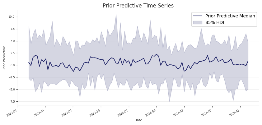
The retained images below come from earlier examples. Their generating
configuration and seed are not recorded here, so they are not reproducible
outputs of the preceding 94% call. Use their captions and legends to identify
the displayed interval and scale.
The first image shows a predictive median and a band labelled 85% HDI. Its
vertical axis has values around 0.2–0.8 and does not identify the target units.
The code above requests 94%; do not use this image as its expected interval or
infer original-scale business values from the axis.
The second image shows observed values and a fitted mean on a target axis
marked 1e6, with a band labelled 94% interval. It uses a different displayed
scale from the first image; no conversion between the two is established
here. Inspect systematic misses and the relationship between observations and
the predictive band. The displayed in-sample metrics do not establish
holdout performance or causal validity.
mmm.summary.posterior_predictive() returns a table with:
observed target values
posterior predictive mean and median
HDI bound columns such as abs_error_94_lower and abs_error_94_upper
You can also access the predictive draws directly:
sample_posterior_predictive(...) does not take y. For a holdout or future
window, keep the actual target outside the model and align it yourself if you
want external evaluation.
Use include_last_observations correctly
Set include_last_observations=True when the forecast window needs lag history
for adstock carryover.
When enabled, Abacus:
prepends the last adstock.l_max training observations internally
samples posterior predictive values on the padded data
removes the prepended rows from the returned result
This only works when the input dates do not overlap with the training dates.
If they do overlap, Abacus raises a ValueError.
Practical guidance
Use the training X for fitted-versus-observed checks.
Use future-only dates for forward prediction.
Use the training-window refit pattern for blocked holdout validation.
Keep combined=True if you want a simpler sample dimension.
Use combined=False if you need explicit chain and draw dimensions.
Call sample_posterior_predictive(...) before using
mmm.diagnostics.predictive_summary() or mmm.summary.posterior_predictive().
Common pitfalls
Calling sample_posterior_predictive(...) without X
Expecting y to be passed into the predictive method
Using include_last_observations=True on dates that overlap with training
data
Forgetting that the returned object is extracted samples, while the stored
idata.posterior_predictive group keeps the native posterior predictive
structure
Contributions and Decomposition
Abacus stores additive contribution terms for fitted PanelMMM models and
exposes them through the data wrapper, summary tables, and plotting suite.
Use this page to inspect media, baseline, control, seasonality, and event
effects. For channel efficiency ratios built from media contributions, see
ROAS and Metrics.
Contribution surfaces
You can work with contributions at three levels.
Surface
Use it for
mmm.data
Raw xarray contribution samples
mmm.summary
DataFrames with posterior means, medians, and HDIs
mmm.plot
Time-series and waterfall visualisations
Read raw contribution samples
The lowest-level accessor is mmm.data.get_contributions(...):
Depending on the fitted model, the returned dataset can contain:
channels
baseline
controls
seasonality
events
baseline includes the intercept contribution and any legacy Mundlak
contribution when the fitted model uses use_mundlak_cre=True. For the named
CRE preset, the structured pipeline reports the CRE adjustment separately and
retains it on the baseline or non-incremental side of the decomposition.
identifying columns such as date, channel, control, and any panel
dims
mean
median
HDI bound columns such as abs_error_94_lower and abs_error_94_upper
mmm.summary.contributions(...) does not expose event effects. For event
effects, use mmm.data.get_contributions(include_events=True) or
mmm.summary.mean_contributions_over_time().
Create a wide decomposition table
Use mmm.summary.mean_contributions_over_time(...) when you want one row per
time point and panel slice:
Use original_scale=True when you want business-unit interpretation.
Use mmm.summary.contributions(...) for tidy per-component tables.
Use mmm.summary.mean_contributions_over_time() for decomposition exports.
Use mmm.summary.total_contribution() when you only need component-level
totals.
Common pitfalls
Expecting mmm.summary.contributions(...) to include event effects
Forgetting that baseline can include more than the intercept when legacy
Mundlak CRE is enabled, or that the named CRE adjustment is non-incremental
Using frequency="all_time" with mean_contributions_over_time() or
change_over_time()
Response Curves
Use response curves to inspect the fitted media transformations directly.
Abacus exposes posterior saturation and adstock curves through both the fitted
model and mmm.summary. For decomposition of realised contributions over time,
see Contributions and Decomposition.
Sample saturation curves
Use sample_saturation_curve(...) on a fitted PanelMMM:
The adstock curve is the fitted decay pattern for an impulse of size
amount. It does not use an original_scale option because the returned
weights are not target-unit contributions.
Runner-generated direct contribution artefacts
If you use the retained pipeline runner, Stage 60_response_curves also writes
a forward-pass direct contribution artefact alongside the saturation and
adstock transformation curves:
forward_pass_contribution_curve.nc
forward_pass_contribution_curve_summary.csv
forward_pass_contribution_curve.png
This artefact is different from the saturation-only curve:
the saturation-only curve shows the fitted saturation transform itself
the forward-pass direct contribution curve runs spend through the full fitted
model path, including adstock and saturation
The retained Stage 60 forward-pass plot uses one explicit scenario so the curve
is interpretable: it rescales the full observed historical spend path from
0% to 200%, then plots total channel spend against total channel
contribution in original units. The marker at 100% highlights the fitted
total contribution for the observed historical spend path.
These methods return DataFrames with posterior mean, median, and pointwise
HDI bounds. A sample axis uses the same HDI calculation as chain/draw;
these intervals are not simultaneous bands for the entire curve. See
Summary interval semantics
for the single-interval definition and the correction to earlier equal-tailed
curve summaries.
saturation_curves(...) includes an x column. adstock_curves(...) uses
time since exposure.
MMMSummaryFactory requirement
Curve summaries need access to both the fitted data and the fitted model
transformations.
mmm.summary already satisfies that requirement. If you construct
MMMSummaryFactory manually, pass model=mmm:
These are direct ratios built from fitted media contributions and the model’s
channel inputs, stored as constant_data.channel_data. Abacus does not look
up a separate monetary spend series or convert exposures to spend.
With original_scale=True, the financial interpretations require:
Ratio
Required units
Interpretation
contribution / channel input
Revenue and monetary spend in a common currency
ROAS: revenue per unit of spend
channel input / contribution
Monetary spend and a conversion-count target
Cost per conversion: currency per conversion
Use consistent currency, time periods and panel aggregation for both sides of
the ratio. For example, £200 of contribution divided by £100 of spend gives
ROAS 2; £200 divided by 1,000 impressions gives £0.20 per impression, not ROAS.
If contributions are left on the scaled target space, the result is not in
original business units.
These are model-conditional contribution ratios. Their posterior intervals do
not establish incremental causal returns; see
Causal Identification.
The arrays are element-wise over time, channel, and any panel dims, with
posterior sample dimensions on top.
Abacus returns NaN when it would otherwise divide by zero.
Summarise ROAS
Use mmm.summary.roas(...) for a tidy summary table:
This is the same retained summary surface that mmm.summary.efficiency() uses
for target_type="conversion".
Use the default efficiency metric
Abacus chooses the default efficiency metric and label from the target type.
This selects an accessor; it does not validate currency or convert channel
inputs to spend. The financial labels below require the units stated above:
Use channel_spend() when you want the raw channel-input table with no posterior
aggregation:
spend_df=mmm.summary.channel_spend()
This returns the observed channel inputs with columns such as date, channel,
panel dims, and channel_data. They represent spend only when the model’s
channel inputs are monetary amounts.
Predictive error metrics
Predictive metrics live under mmm.diagnostics.predictive_summary():
These metrics are calculated from the stored posterior predictive samples and
the observed target. See the canonical
predictive metric definitions,
including the observed-range denominator for NRMSE/NMAE and its constant-target
NaN case.
Practical guidance
Use roas() for revenue targets with monetary channel inputs in a common currency.
Use cost_per_target() for conversion-count targets with monetary channel inputs.
Use efficiency() when you want target-type-aware reporting.
Sample posterior predictive values before using predictive metrics.
Common pitfalls
Reporting revenue per exposure as ROAS because a channel input was labelled
spend without checking its units
Forgetting that zero spend or zero contribution produces NaN
Using predictive diagnostics before calling
sample_posterior_predictive(...)
Summary and Export
mmm.summary is the retained tabular summary surface for fitted PanelMMM
models.
It is backed by MMMSummaryFactory and returns pandas or polars DataFrames
that you can export with normal DataFrame methods.
For predictive diagnostics and JSON-ready reports, see
Diagnostics.
Use mmm.summary
The simplest path is the bound summary factory on the fitted model:
Summary tables include interval columns named from those probabilities. For
example, hdi_probs=[0.94] produces columns such as:
abs_error_94_lower
abs_error_94_upper
These columns contain interval endpoints, not error magnitudes. Abacus uses
ArviZ’s single contiguous empirical HDI for both chain/draw and sample
layouts. Reshaping the same draws does not change the bounds. Means, medians,
coordinate labels and output column names are independent of that layout.
NaNs are not silently removed before calculating the HDI; inspect non-finite
bounds before interpreting or exporting them.
Each interval summarises one output coordinate. Curve intervals are pointwise,
not simultaneous bands over a whole response curve. A single contiguous
interval also need not represent a disconnected highest-density set for a
multimodal posterior.
Earlier versions used equal-tailed quantiles for arrays with a sample
dimension, including curve summaries. Those bounds can differ materially from
HDIs for skewed draws. Recompute affected tables from the same saved draws to
obtain consistent HDIs; no refit is required. Means, medians and column names
remain unchanged.
Blocked holdout coverage
uses equal-tailed predictive intervals. Its coverage_* fields do not measure
coverage of these HDI columns.
Aggregate over time
Many summary methods accept frequency with one of these values:
Expecting a dedicated file-export API on mmm.summary
Passing 94 instead of 0.94 in hdi_probs
Using saturation_curves() or adstock_curves() from a manual factory
without model=mmm
Using all_time on summaries that require a date dimension
Optimisation
This section covers Abacus budget optimisation workflows for fitted
PanelMMM models. It explains the low-level optimisation wrapper, how to
inspect optimisation outputs.
For the higher-level planner service and Dash UI, see
Scenario Planning.
Pages
Budget Optimisation - How to run
PanelBudgetOptimizerWrapper, set bounds and masks, and define spend over a
future window.
Interpreting Optimisation - How to read the
allocation output, inspect simulated response samples, and use the pipeline
optimisation artefacts.
Scenario Planning - How to compare current, manual,
and fixed-budget optimised scenarios with the planner service and optional
Dash UI.
Subsections of Optimisation
Budget Optimisation
Use PanelBudgetOptimizerWrapper when you want to optimise spend for a fitted
PanelMMM over a future date window.
The wrapper rejects the named FE, CRE and release-gated RE presets with
EstimatorOperationError. Use the
estimator support matrix
before preparing an optimisation. FE/CRE historical and manual scenarios are
separate supported operations; they do not enable fixed-budget optimisation.
The wrapper builds a synthetic future dataset for the requested window, swaps
the model’s channel_data for an optimisation variable, and then calls the
generic BudgetOptimizer. If you want to compare several plans in total
horizon spend units, see Scenario Planning.
What the optimiser maximises
For PanelBudgetOptimizerWrapper, optimize_budget() defaults to:
The optimiser therefore maximises the average posterior response of the chosen
response variable, subject to your budget bounds and constraints.
Budget units
The low-level wrapper uses per-period spend units.
budget is the total spend across all optimised cells for one model period.
The returned allocation has no date dimension, so Abacus repeats that
allocation across the optimisation window.
If the window has num_periods=8 and you pass budget=100_000, the
simulated spend over the full horizon is 800_000 before any carryover
effects are applied.
This is different from Scenario Planning, which
treats total_budget and manual allocations as total horizon spend and
converts them to per-period units internally.
The structured pipeline now has two YAML paths:
preferred: optimization.budget, which uses total horizon spend and is
converted internally before calling the wrapper
legacy: optimization.total_budget, which keeps the old per-period spend
contract for backward compatibility
Required inputs
Input
What Abacus expects
Notes
model
A fitted PanelMMM with idata.posterior
The optimiser needs posterior draws and model graph variables.
start_date, end_date
A future window at the model’s observed date frequency
Abacus infers num_periods from the training data frequency.
allocation is an xarray.DataArray over the non-date budget dimensions.
For a model with dims=("geo",), the result dims are typically
("geo", "channel").
Bounds and masks
budget_bounds
Use budget_bounds to cap spend for each optimised cell.
If the budget has only one non-date dimension, you can pass a dict such as
{"tv": (0.0, 50_000.0), "search": (0.0, 30_000.0)}.
For panel budgets, pass an xarray.DataArray with dims
(*budget_dims, "bound"), where "bound" contains "lower" and "upper".
If you omit budget_bounds, Abacus warns and uses (0, total_budget) for
every optimised cell.
Abacus reindexes DataArray bounds to the model’s internal coordinate order,
so the input coordinate order does not need to match exactly.
budgets_to_optimize
Use budgets_to_optimize to choose which cells can move.
The mask must have boolean dtype and exactly the budget dimensions.
Each budget dimension must have explicit, unique, non-missing coordinate labels
matching the model’s labels exactly. Abacus aligns label and dimension order
before selecting cells. Missing or extra labels raise ValueError.
Unoptimised cells are fixed at zero in the returned allocation.
If you omit the mask, Abacus optimises every cell where the fitted model has
non-zero historical channel_contribution information.
If your mask includes True for a cell where the model has no information,
Abacus raises ValueError.
Time distribution across the window
Use budget_distribution_over_period to flight each allocation cell over time
instead of repeating the same spend every period.
The object must be an xarray.DataArray with:
exactly the dimensions ("date", *budget_dims), in any order
explicit, unique, non-missing labels for every budget dimension, matching the
model’s coordinate membership exactly
one date weight per optimisation period, retained in the supplied date order
finite, real, non-negative fractions that sum to 1 across date for every
budget cell, including cells disabled by the mask
Abacus aligns channel and other budget labels before converting the profiles
to arrays. Reordered labels are accepted; missing, extra, duplicate or absent
budget labels raise ValueError. Valid zero fractions are accepted. Invalid
fractions are rejected, not clipped or normalised. Sum validation uses relative
tolerance 1e-5 and absolute tolerance 1e-8.
Previously saved allocations are not repaired by this validation. Recompute
allocations produced with misordered profiles or invalid fractions.
The low-level optimiser treats the date axis as an ordered sequence and accepts
implicit positional dates. It does not sort or match calendar dates. The
wrapper’s response-simulation date checks are described below.
Use the same budget_distribution_over_period again when you call
sample_response_distribution(),
otherwise you will optimise one spend path and simulate another.
For response simulation through the wrapper, the date coordinates can be:
integer positions 0 .. num_periods - 1, or
exact dates that match the optimisation window
Constraints and solver controls
default_constraints=True adds the default equality constraint:
sum(allocation) == budget
This is enabled by default and emits a warning so you can see that the default
constraint set is active.
You can also pass:
extra SciPy minimise keyword arguments directly to optimize_budget(...) to
tweak the underlying solver call
callback=True to get a third return value with per-iteration objective,
gradient, and constraint diagnostics
YAML note for the pipeline runner
If you run optimisation through the structured pipeline, configure the
optimization block in YAML:
In this preferred pipeline path, optimization.budget is interpreted as total
horizon spend. Abacus resolves the configured budget, divides by
num_periods, scales any derived bounds to per-period units, and then calls
optimize_budget(...).
then optimization.total_budget continues to mean per-period spend.
Common pitfalls
Passing a total horizon budget to optimize_budget(...). Divide by
wrapper.num_periods first, or use the pipeline optimization.budget block
or Scenario Planning.
Mixing up the preferred horizon-based optimization.budget block and the
legacy per-period optimization.total_budget field.
Passing dict bounds for a panel budget. Dict bounds only work when the budget
dims are just ("channel",).
Omitting a budget dimension from budget_distribution_over_period. The
distribution must include every budget dim, not just the one you want to vary.
Forgetting that response_variable must exist in the fitted optimisation
graph.
Using one budget distribution for optimisation and a different one for
response simulation.
allocation is an xarray.DataArray over the non-date budget dimensions.
Model shape
Typical allocation dims
Meaning
No extra panel dims
("channel",)
One optimised value per channel
dims=("geo",)
("geo", "channel")
One value per (geo, channel) cell
dims=("geo", "brand")
("geo", "brand", "channel")
One value per (geo, brand, channel) cell
The values are in the wrapper’s per-period units. Unoptimised cells are
present and set to zero.
result
result is SciPy’s OptimizeResult. The fields you will usually inspect are:
Field
Meaning
success
Whether the solver converged
status
SciPy status code
message
Human-readable solver message
fun
Final objective value
nit
Number of iterations
x
The optimised flat parameter vector
If success is False, Abacus raises MinimizeException unless you opt in to
return_if_fail=True on the underlying BudgetOptimizer.
callback_info
When callback=True, Abacus records one entry per solver iteration. Each entry
includes:
x
fun
jac
constraint_info when constraints are active
Use this when you need to diagnose solver behaviour rather than just consume the
final allocation.
Simulate the optimised plan
The optimiser itself returns only the allocation. To estimate spend paths and
contributions over the requested window, call sample_response_distribution().
Set noise_level=0.0 when you want the spend path to match the requested
allocation exactly.
What response_samples contains
The wrapper builds a synthetic future dataset, samples posterior predictive
draws, and then merges the requested allocation and simulated spend path back
into the result.
response_samples therefore contains:
Variable
Source
Meaning
allocation
Added by the wrapper
Requested allocation without a date dimension
One variable per channel
Added by the wrapper
Simulated spend path over the future dates
mmm.output_var
Posterior predictive sample
Model output variable
channel_contribution
Posterior predictive sample
Channel contribution on model scale
total_media_contribution_original_scale
Posterior predictive sample
Total media contribution on the original target scale
If you pass additional_var_names, Abacus also includes those variables when
they exist in the model graph.
Carryover and evaluation window
include_carryover=True changes how Abacus builds the synthetic future window.
Abacus extends the generated dates by adstock.l_max periods.
It then zeroes the tail spend rows after the requested window.
The extra dates let posterior predictive sampling include lagged effects from
the planned spend.
This is why the simulated dataset can cover a longer evaluated window than the
requested start_date to end_date range, while still preserving the same
total spend.
Plot the result
The plotting helpers under mmm.plot are designed to work directly with the
response dataset returned by the wrapper.
split_by="geo" or another dimension to create separate subplots
original_scale=True to prefer original-scale contribution variables when
they are available
Example optimisation output:
Read the Stage 70 pipeline artefacts
If you run optimisation through python -m abacus.pipeline.runner, Stage 70
writes both the low-level optimiser output and several interpretation files.
The simulated response dataset for that allocation
optimize_result.json
Solver status, message, objective value, and iteration count
budget_summary.csv
Current versus optimised totals
budget_response_points.csv
Per-channel current versus optimised spend, contribution, and efficiency summaries
budget_impact.csv
Delta between current and optimised channel summaries
budget_bounds_audit.csv
Current spend, scaled reference spend, bounds, optimised spend, and bound checks
budget_roi_cpa.csv
Channel efficiency summaries using the model’s efficiency metric
budget_response_curves.csv
Saturation-only response curve summaries
budget_mroi.csv
Marginal efficiency estimates at the current and optimised spend points
The stage also writes plots for allocation, contribution over time, response
curves, impact, bounds audit, and ROI or CPA summaries.
These Stage 70 spend figures are reported in total horizon spend units so they
can be compared directly to current historical spend over the same reference
window. Abacus still converts to the low-level wrapper’s per-period budget
contract internally.
Practical checks
Before you use an optimised plan, check:
result.success and result.message
whether the allocation matches your intended budget units
whether budget_bounds_audit.csv or your own checks show any bound issues
how much of the gain comes from reallocation versus carryover assumptions
whether the point lies on a sensible part of the response curve, not just on
the edge of a bound
For multi-plan comparison in total horizon units, use
Scenario Planning.
Use this section when you want to compare historical, manual, and optimised
future plans with abacus.scenarios.
The scenario planner is a higher-level planning surface than the low-level
optimisation wrapper. It works in total horizon spend units, returns
versioned structured comparison tables, and supports Python and CLI workflows.
abacus.scenario_planner remains the legacy compatibility namespace for
existing statistical imports and advisory dashboard facades. The experimental
abacus-dashboard application is deprecated. Its retained guide documents
historical behaviour; use abacus.scenarios for current workflows.
Pages
Supported Surface: The recommended scenario entry
points, compatibility facades, fitted-run contract, persisted workspace
state, and estimator limits.
Overview and Workflow: What the planner does,
how it differs from low-level optimisation, and how scenario windows work.
Scenario Specifications: The public scenario
spec classes, versioned YAML recipes, allocation shapes, bounds, and budget
distributions.
Python API: How to use ScenarioPlanner.evaluate(...) and
run retained recipes from Python, plus the compatibility workspace helpers.
Comparison Outputs: The structure and meaning of
ScenarioResult, ScenarioComparison, retained artefacts, and the dashboard
payload contract.
Historical reference
Deprecated Dash App: Retained documentation for the
experimental dashboard. It is not a recommended scenario workflow.
Subsections of Scenario Planning
Overview and Workflow
Use the scenario planner when you want to compare whole plans rather than run a
single low-level optimisation call.
The planner combines typed scenario specifications, a Python comparison
service, and a CLI for retained YAML recipes. Use abacus.scenarios for
scenario workflows. The experimental abacus-dashboard application is
deprecated; its legacy import facades remain in this checkout.
For supported entry points and estimator limits, see
Supported Surface.
What the planner compares
The retained planner supports three scenario types:
Scenario type
Purpose
Public spec
Current
Use observed history as a reference plan
CurrentScenarioSpec
Manual allocation
Simulate a user-defined future plan
ManualAllocationScenarioSpec
Fixed-budget optimised
Optimise a future plan at a fixed budget
FixedBudgetOptimizedScenarioSpec
Planner units versus optimiser units
The most important distinction is budget units.
Surface
Public budget contract
PanelBudgetOptimizerWrapper
Per-period spend
abacus.scenarios.ScenarioPlanner
Total spend over the whole scenario horizon
For example, if a four-period scenario has a total budget of 900_000, the
planner converts that to per-period units internally before it calls the
wrapper or response sampler.
Requested and evaluated windows
Each scenario has a requested window from start_date to end_date.
For simulated scenarios, the evaluated window can be longer than the requested
window when you set include_carryover=True. Abacus extends the synthetic
future path so lagged adstock effects can continue after the requested end
date.
The planner reports both windows in the metadata output.
Historical overlap for current scenarios
CurrentScenarioSpec is strict about history.
Its requested window must overlap observed data. Abacus does not reinterpret a
future-only window as “use the latest history instead”.
Typical workflow
The common workflow is:
Fit PanelMMM.
Build one or more scenario specs.
Run abacus.scenarios.ScenarioPlanner.compare(...), or evaluate a YAML
recipe against a fitted run with python -m abacus.scenarios.
Inspect the comparison tables, save workspaces, and export the planning
outputs you need.
Mixing up total horizon spend and per-period spend
Using a future-only window in CurrentScenarioSpec
Forgetting that carryover can extend the evaluated window
Scenario Specifications
This page documents the public spec classes under abacus.scenarios.
abacus.scenario_planner still re-exports these classes for compatibility
with existing imports, but new code should use abacus.scenarios.
Most users create one of the three concrete scenario specs:
CurrentScenarioSpec
ManualAllocationScenarioSpec
FixedBudgetOptimizedScenarioSpec
Abacus also exposes shared base models such as
HistoricalReferenceScenarioSpec and SimulatedScenarioSpec, but you do not
normally instantiate those directly.
The named FE and CRE presets support historical and manual scenarios for the
complete set of fitted units; CRE also retains its frozen fitted summaries.
They do not support FixedBudgetOptimizedScenarioSpec. The RE preset remains
release-gated. Check the
estimator support matrix
before choosing a scenario type.
Shared fields
All public scenario specs inherit these core fields:
Field
Meaning
name
Display name for the scenario
start_date
Requested scenario start date
end_date
Requested scenario end date
scenario_id
Stable scenario key used in outputs
If you do not set scenario_id, Abacus derives one by slugifying name.
Scenario IDs must be unique within one ScenarioPlanner.compare(...) call.
CurrentScenarioSpec
Use CurrentScenarioSpec for a historical reference plan.
Abacus materialises DataArraySpec as an xarray.DataArray before it
validates dims and coordinates.
Versioned scenario recipes
Use ScenarioRecipe to retain several scenario specifications as one
versioned request. The recipe contract rejects unknown versions, empty
scenario lists, duplicate scenario IDs, and unknown top-level fields.
Abacus writes a new immutable evidence directory under
<fitted-run>/scenario_planner/recipes/. It does not refit the model or alter
the fitted run manifest.
Common pitfalls
Reusing the same scenario_id twice in one comparison
Using dict allocations or dict bounds for panel budgets
Passing an allocation or bounds object with missing coordinates
Providing a budget_distribution_over_period that does not sum to 1
Reusing an existing recipe output directory; retained evidence is never
overwritten
Python API
Use ScenarioPlanner when you want to evaluate one scenario or compare
multiple scenarios from Python.
The preferred public API lives under abacus.scenarios.
abacus.scenario_planner remains available for existing statistical
compatibility imports, but new statistical scenario code should use
abacus.scenarios. The experimental abacus-dashboard application is
deprecated; dashboard helpers below are historical reference only.
For the recommended entry points and current scope, see
Supported Surface.
Prerequisite
ScenarioPlanner requires a fitted PanelMMM with idata.
If you construct the planner before fitting, Abacus raises ValueError.
The named FE and CRE presets support historical and manual scenarios for the
complete set of fitted units; CRE also retains its frozen fitted summaries.
They do not support FixedBudgetOptimizedScenarioSpec. The RE preset remains
release-gated. Check the
estimator support matrix
before choosing a scenario type.
These helpers belong to the deprecated experimental dashboard. This section
records the former abacus_dashboard.app interface for existing integrations;
it is not a recommended workflow for new code.
Helper
What it returns
Use it when
load_workspace_bundle(...)
run_context, workspace_service, workspace
you want the fitted run context and active workspace without starting Dash
create_app_from_results_dir(...)
app, run_context, workspace_service, workspace
you want to launch or embed the dashboard app from Python
These helpers expect a fitted results directory with run_manifest.json and a
fit-stage idata artefact.
When available, the loader rebuilds the model from in-run metadata config
artifacts in this order:
00_run_metadata/config.resolved.yaml
00_run_metadata/config.original.yaml
the copied config file under 00_run_metadata/
run_manifest.json["config_path"] as fallback
The returned run_context records both config_path and
config_provenance_type so callers can tell which source was used.
Residual portability risk remains if the chosen config still points to dataset
files outside the saved run directory.
Legacy imports from abacus.scenario_planner still resolve for compatibility
and emit advisory DeprecationWarnings. No legacy dashboard app-layer facade
will be removed before Abacus 4.0.
Evaluate one scenario
Use evaluate(...) when you want one scenario result:
Unlike ScenarioResult, the combined object uses the plural
allocations.
Run a versioned recipe
Use ScenarioRecipe for an in-memory Python request. Use
load_scenario_recipe(...) for YAML and run_scenario_recipe(...) when the
model has already been retained by the pipeline.
The default output path is a new timestamped directory under
scenario_planner/recipes/ in the fitted run. Pass output_dir= only when you
need another new location. Abacus rejects an existing target directory so a
later evaluation cannot silently replace retained evidence.
Use evaluate_scenario_recipe(...) when you already have the fitted model in
memory:
This example creates the default workspace if it is absent. Use
load_workspace(...) instead when you require a specific existing workspace
ID.
WorkspaceService defaults to synchronous jobs when you instantiate it
directly. The dashboard app uses ThreadedScenarioPlannerJobRunner through
the dashboard compatibility layer.
Prepare data for a client UI
Use to_store_payload() when you want a JSON-friendly version of the
comparison tables:
payload=comparison.to_store_payload()
This method converts datetime columns to YYYY-MM-DD strings and returns a
dict with a scalar contract_version plus record lists for the comparison
tables. Compare contract_version with SCENARIO_CONTRACT_VERSION before a
dashboard or external client assumes a payload shape.
Background-job helpers
For custom integrations, WorkspaceService also exposes queue/apply methods:
submit_draft_evaluation(...)
apply_draft_evaluation_job(...)
submit_sensitivity_sweep(...)
apply_sensitivity_sweep_job(...)
Use these only when you need the same background-job pattern as the current
dashboard beta. For most scripted flows, the blocking methods are simpler.
Relationship to the low-level wrapper
ScenarioPlanner uses PanelBudgetOptimizerWrapper internally for simulated
scenarios, but its public contract is different:
you pass total horizon budgets and allocations
the planner converts them to per-period units internally
the planner returns comparison tables rather than raw optimiser objects
If you want direct access to optimize_budget(...) or
sample_response_distribution(...), use
Budget Optimisation instead.
Common pitfalls
Passing per-period spend into ManualAllocationScenarioSpec or
FixedBudgetOptimizedScenarioSpec
Expecting duplicate scenario_id values to be allowed in compare(...)
Forgetting that result.allocation and comparison.allocations use
different attribute names
Comparison Outputs
ScenarioPlanner returns structured planning tables rather than a single
optimiser object.
This page explains the output objects and the meaning of each table.
Import these objects from abacus.scenarios for new statistical scenario
code. abacus.scenario_planner remains a compatibility namespace for existing
statistical imports and legacy dashboard app-layer paths.
ScenarioComparison is a row-wise concatenation of the individual scenario
results, with scenario identifiers added to every table.
totals
totals has one row per scenario.
It includes:
scenario_id
scenario_name
scenario_type
total_spend
contribution_mean
contribution_median
contribution_hdi_94_lower
contribution_hdi_94_upper
efficiency_metric
efficiency_mean
efficiency_median
efficiency_hdi_94_lower
efficiency_hdi_94_upper
efficiency_metric is ROAS for revenue targets and CPA for conversion
targets.
channels
channels has one row per (scenario, channel).
It includes:
scenario identifiers
channel
spend
spend_share
spend_per_period
contribution summary columns
contribution-per-period columns
efficiency summary columns
efficiency_metric
The planner aggregates non-channel panel dims before it builds this table. For
example, a (geo, channel) model still returns one row per channel here.
contributions_over_time
contributions_over_time has one row per (scenario, date, channel).
It includes:
scenario identifiers
date
channel
contribution_mean
contribution_median
contribution_hdi_94_lower
contribution_hdi_94_upper
Like channels, this table aggregates non-channel panel dims before
summarising.
allocations
allocations keeps the original allocation grain.
It includes:
scenario identifiers
the allocation dims, such as channel, geo, or brand
allocation
realized_spend
For current scenarios, allocation is the summed historical spend over the
reference window. For simulated scenarios, allocation is the requested total
horizon allocation and realized_spend is the realised spend from the response
simulation.
metadata
metadata is the audit table for each scenario.
Shared fields include:
scenario_id
scenario_name
scenario_type
start_date
end_date
evaluated_start_date
evaluated_end_date
num_periods
target_type
efficiency_metric
Additional fields depend on scenario type.
Current scenario metadata
Current scenarios add:
reference_window_dates
Manual scenario metadata
Manual scenarios add:
requested_total_budget
total_budget
reference_window_dates
budget_unit
Fixed-budget optimised metadata
Optimised scenarios add:
requested_total_budget
total_budget
optimization_success
optimization_status
optimization_message
optimization_objective_value
reference_window_dates
budget_unit
Requested versus evaluated windows
The metadata table is the best place to check whether the evaluated window
matches the requested window.
When include_carryover=True, the evaluated end date can be later than the
requested end_date.
ScenarioComparison.to_store_payload() converts the comparison tables into a
JSON-friendly dict:
payload=comparison.to_store_payload()
The payload contains a scalar contract_version and record lists for
totals, channels, contributions_over_time, allocations, and
metadata. The current contract value is exported as
SCENARIO_CONTRACT_VERSION from abacus.scenarios, so downstream clients can
check whether they understand the result shape before rendering or importing
it.
The deprecated experimental abacus-dashboard application consumed this
payload format. The versioned contract remains available to machine consumers:
Abacus owns the statistical result shape; clients own rendering and interaction.
Retained recipe artefacts
run_scenario_recipe(...) and evaluate_scenario_recipe(...) persist the
comparison as an immutable bundle:
File
Purpose
scenario_recipe.resolved.yaml
versioned request after validation
scenario_validation.json
scenario IDs, estimator, fitted-unit scope, estimand, and pass state
estimator_manifest.yaml
fitted estimator contract copied with the scenario evidence
scenario_totals.csv
total spend, contribution, efficiency, and uncertainty by scenario
scenario_channels.csv
channel summaries and uncertainty
scenario_contributions_over_time.csv
date-channel contribution summaries and uncertainty
scenario_allocations.csv
requested allocation and realised spend at the original allocation grain
scenario_metadata.csv
scenario semantics, dates, history policy, scale, and estimand
scenario_payload.json
versioned five-table payload for machine consumers
scenario_artifact_manifest.json
source run ID, file sizes, and SHA-256 checksums
The target directory must not exist before evaluation. Abacus validates the
comparison before it creates the directory and never overwrites an earlier
bundle.
Common pitfalls
Reading channels as if it retained non-channel panel dims
Ignoring metadata when carryover is enabled
Comparing requested allocation with realised spend without checking the
allocations table
Supported Surface
Use abacus.scenarios for supported Python and CLI scenario workflows.
The experimental abacus-dashboard application is deprecated. It is not a
recommended entry point.
Legacy dashboard app-layer imports under abacus.scenario_planner remain as
advisory compatibility facades in this checkout. Their warnings identify
abacus_dashboard.* paths; those paths belong to the deprecated application.
Estimator prerequisites
The named FE and CRE presets support historical and manual scenarios for the
complete set of fitted units; CRE also retains its frozen fitted summaries.
They do not support FixedBudgetOptimizedScenarioSpec. The RE preset remains
release-gated. Check the
estimator support matrix
before choosing a scenario type.
Dashboard compatibility code does not add estimator support.
Recommended entry points
Use these entry points in preference order.
Entry point
Use it when you want to
Notes
abacus.scenarios.ScenarioPlanner
evaluate or compare scenarios from Python
Preferred statistical API for notebooks, scripts, and testable planning flows
python -m abacus.scenarios
evaluate a YAML recipe against a fitted run
Writes an immutable, checksummed evidence bundle under the fitted run
abacus.scenarios.run_scenario_recipe(...)
run the same retained recipe workflow from Python
Preferred scripted handoff when the fitted model is already saved
abacus.scenarios.WorkspaceService
work with saved workspaces programmatically
Library-facing surface for cloning, saving, evaluating, sweeping, and exporting
Advanced integration surfaces
Abacus exposes lower-level statistical orchestration objects such as:
ThreadedScenarioPlannerJobRunner
SynchronousScenarioPlannerJobRunner
WorkspaceStore
These are public, but they are more implementation-shaped than the recommended
entry points above. Use them only when you need to override job-runner or
storage behaviour.
Results directory contract
The dashboard-specific sections below record the deprecated prototype,
including its former compatibility plans. They do not recommend launching it
or establish a future release commitment. The statistical recipe and workspace
APIs remain available through abacus.scenarios.
The dashboard launcher and load_workspace_bundle(...) expect a fitted run
directory, not raw modelling inputs.
The run directory must include:
Requirement
Why it matters
run_manifest.json
Abacus uses it to locate the config and saved artefacts
a fit-stage idata artefact
Abacus attaches the saved posterior to the rebuilt model
When metadata-stage config artefacts are present, Abacus prefers those
in-run files when rebuilding the saved PanelMMM:
00_run_metadata/config.resolved.yaml
00_run_metadata/config.original.yaml
the copied config file under 00_run_metadata/
Only when those in-run config artefacts are absent does the planner fall back
to run_manifest.json["config_path"].
That makes the compatibility loader more portable when the original config
path is no longer available, but it does not guarantee full relocation across
machines. The chosen config can still reference dataset files outside the run
directory.
The planner can also load these optional optimisation artefacts when they are
present:
70_optimisation/budget_response_curves.csv
70_optimisation/budget_bounds_audit.csv
When these files are available, the app can show saved saturation-reference
response-curve and bounds-audit views.
Companion dashboard handoff contract
A retained recipe writes scenario_payload.json for machine consumers. The
companion abacus-dashboard package must:
reject a missing or unknown contract_version;
compare that value with SCENARIO_CONTRACT_VERSION before rendering;
preserve all five record collections: totals, channels,
contributions_over_time, allocations, and metadata;
use scenario_validation.json, estimator_manifest.yaml, and
scenario_artifact_manifest.json as provenance and integrity evidence; and
label the outputs as posterior media contributions, not total outcomes,
profits, causal effects, or model approval.
Abacus owns this statistical payload. The companion package owns rendering,
interaction, and any application persistence. This repository does not add or
change dashboard UI code as part of the recipe workflow.
The companion package also provides a read-only bundle viewer. It verifies the
manifest checksums for every declared artifact and requires agreement among
the payload, validation record, and estimator manifest before it renders the
five collections. It rejects tampered or incompatible bundles rather than
attempting a partial display.
What the app persists
The workspace app stores its own planning state under the fitted run
directory:
Deprecated experimental application. Use the abacus.scenariosPython API or recipe CLI for
current scenario workflows.
The rest of this page is a historical record of the abacus-dashboard
prototype. Installation commands, launch procedures, screenshots, beta limits
and compatibility plans below describe that prototype, not a current product
recommendation or release commitment.
The app does not fit PanelMMM. It loads an existing fitted run, reuses the
saved idata, and evaluates planner scenarios against that fitted model.
For the current statistical API and estimator limits, see
Supported Surface.
Interface version and screenshots
This guide describes the workspace interface in the companion source declaring
abacus-dashboard version 0.1.0a0, checked on 24 September 2026. The five-page
navigation and the Explain → Diagnostics and audit section were checked
against that source. This identifies the documented interface; it does not
certify an installed build or a published release.
The screenshots below show an earlier read-only demonstration interface with
four navigation entries. Their exact app version was not recorded. They are
historical illustrations, not screenshots of the documented five-page
workspace. Follow the page names and procedures in the text.
Legacy app-layer imports and launchers under abacus.scenario_planner still
work as advisory compatibility facades, but new dashboard code should use
abacus_dashboard.*.
This launcher is the workspace entry point for beta evaluation. It
loads the fitted run, opens or seeds a planner workspace, and starts the app
with the threaded job runner used by the UI.
To inspect a retained YAML-recipe result without opening or creating a
workspace, use the mutually exclusive read-only evidence-review mode:
Before the dashboard renders, this mode verifies every manifest checksum and
cross-checks the versioned payload, scenario validation evidence, and fitted
estimator manifest. It renders all five retained record collections. It does
not fit, refit, evaluate, optimise, mutate evidence, or infer total outcomes,
profits, causal effects, or model approval.
Useful flags:
--workspace-id to open one previously saved workspace
--workspace-name to control the seeded workspace name
--current-periods and --future-periods to change the default seeded windows
--budget-scale to scale the default future budget
--build-only to validate the run and print a summary without starting Dash
--host, --port, and --debug for the Dash server
--workspace-id, --workspace-name, --current-periods, --future-periods,
and --budget-scale apply only with --results-dir. The evidence-review mode
rejects them rather than silently ignoring them.
The dashboard package also exposes the lower-level
create_scenario_planner_dash_app(...) factory when you already have a
ScenarioComparison or ScenarioWorkspace.
New statistical scenario code should use abacus.scenarios. Legacy
abacus.scenario_planner app-layer imports remain available as advisory
compatibility facades and emit DeprecationWarnings that name the replacement
abacus_dashboard.* import.
What the launcher requires
The dashboard launcher expects a fitted results directory that contains:
run_manifest.json
a fit-stage idata artefact
When the metadata stage is present, the launcher prefers the in-run config
artefacts under 00_run_metadata/ and only falls back to
run_manifest.json["config_path"] if those files are absent.
In build-only mode, the launcher prints the selected config path and its
provenance so you can see whether the planner loaded:
resolved_in_run
original_in_run
copied_in_run
external_manifest_path
This makes the launcher more portable when the original config path no longer
exists, but the chosen config can still fail if it references dataset files
that are not present on the current machine.
When these optional files are present, the app also loads them for richer UI
views:
70_optimisation/budget_response_curves.csv
70_optimisation/budget_bounds_audit.csv
What the UI includes
The documented workspace interface has five pages:
Plan Setup for run context, workspace metadata, saved workspaces, draft inventory, and the launch path into Scenario Builder
Scenario Builder for editing one draft at a time and evaluating it back into the workspace
Review for cross-scenario totals, deltas, rankings, movers, and approval/export readiness
Explain for response curves, operating-region views, lift comparisons, and diagnostics/audit surfaces
Export for reproducible export bundles and deterministic sensitivity output selection
What the app saves
The workspace app persists planning state under the fitted run directory:
Path
What Abacus saves
scenario_planner/workspaces/
workspace JSON files and compact manifests
scenario_planner/cache/
cached evaluated scenarios and cache index
scenario_planner/exports/
export bundles and zipped archives
This means a planner session stays attached to one fitted run.
Plan Setup page
The Plan Setup page shows the loaded run context and the active planner
workspace. It also lets you:
open a different saved workspace for the same run
clone the current workspace into a new planning branch
edit workspace name, owner, tags, and notes
inspect revision history, job history, and evaluation-cache reuse
launch the current workspace into Scenario Builder
This page is the planner launch surface: planning context stays visible first,
while operational details remain available through collapsed secondary
sections.
Scenario Builder page
The Scenario Builder page is interactive. You can:
create current, manual_allocation, and fixed_budget_optimized drafts
duplicate or delete drafts
edit names, dates, carryover, budget, and manual allocations
capture scenario owner, workflow status, approvals, pinning, tags, and notes
evaluate and save the draft back into the workspace
When a draft has been evaluated, the page shows planned versus realised spend,
allocation detail, and scenario metadata. When a draft has changed but has not
yet been re-evaluated, the page shows a draft preview instead.
Historical illustration of allocation review:
Earlier demonstration interface; exact version unrecorded. This view compares
planned allocation with realised spend and shows requested and evaluated
windows. It does not illustrate the current draft-editing controls. Use the
workspace’s Scenario Builder procedure above for editing and evaluation.
Review page
The Review page focuses on scenario-to-scenario trade-offs and review
readiness. It includes:
scenario summary cards
overview and delta charts
channel comparison charts
scenario ranking and top-mover tables
contribution-over-time comparisons
Historical illustration of scenario comparison:
Earlier demonstration interface; exact version unrecorded. Its Compare
Scenarios page illustrates totals and differences relative to a baseline.
In the documented workspace, use Review for this task. These displayed
example values are not evidence that a proposed allocation improves outcomes.
Explain and Export pages
The remaining pages build on the same workspace state:
Explain overlays scenario reference points on the saved Stage 70 saturation-only response-curve artefact when available
the plotted marker position follows the saved reference curve at each scenario’s spend-per-period level
marker hover text also shows the actual evaluated average contribution so you can compare the scenario outcome with the reference-curve position
Explain also surfaces scenario warnings, optimiser status, bounds audit, allocation reconciliation, operating-region views, and lift comparisons
Export writes reproducible bundles under the run directory and exposes any saved sensitivity output selections
Background jobs
The dashboard app runs draft evaluation and sensitivity sweeps as background
jobs.
In this beta:
the app queues draft evaluation and sensitivity sweeps
the UI polls the active job and refreshes the workspace when the job completes
export runs synchronously, but Abacus still records it in job history
The UI currently tracks one active planner job at a time. Finish the current
evaluation or sweep before starting another one.
Practical guidance
Launch the app from a fitted results directory, not from raw input data.
Use separate cloned workspaces for competing planning narratives.
Re-evaluate a draft after changing dates, budget, or allocation values.
Check both requested and evaluated windows when carryover is enabled.
Open Explain → Diagnostics and audit before exporting or sharing a
scenario set. Diagnostics is a historical screenshot label, not a separate
page in the documented workspace.
Treat the dashboard launcher as a local beta workflow rather than a
production deployment surface.
Use abacus-dashboard as the dashboard app home; treat
abacus.scenario_planner dashboard paths as legacy compatibility.
Legacy compatibility window
Compatibility remains advisory with no removal before Abacus 4.0. Removal of
legacy dashboard app-layer facades under abacus.scenario_planner also
requires:
a documented abacus-dashboard release and install path
passing dashboard smoke checks against the supported Abacus scenario contract
zero known internal imports using legacy dashboard paths
Common pitfalls
Launching the app without installing the companion abacus-dashboard package
Pointing the launcher at a directory without run_manifest.json and fit artefacts
Expecting the app to fit a model from scratch
Interpreting a draft preview as evaluated output before clicking Evaluate and Save
Starting a second evaluation or sweep while another planner job is still running
Pipeline Runner
This section covers the structured abacus.pipeline runner: how it loads a
config and dataset, executes the retained stage sequence, and writes
reproducible run artefacts to disk.
Pages
Runner Overview - How run_pipeline(...) works, which
stages run, and when the optimisation stage is skipped.
YAML Configuration - Which YAML keys the runner
consumes and how they map to model build, data loading, holidays, and
optimisation.
Blocked Holdout Validation - What Stage 35
does, how to configure it, and how to read the holdout metrics and plots.
CLI Reference - The thin python -m abacus.pipeline.runner
interface and its supported flags.
Output Directory Schema - The run directory
layout, manifest schema, stage statuses, and main artefacts.
Extending the Runner - How to add a stage or wire
in reporting without bypassing the manifest and artifact helpers.
Subsections of Pipeline Runner
Runner Overview
Use the pipeline runner when you want a full disk-backed PanelMMM run instead
of only an in-memory fit.
The runner loads a YAML config and a CSV dataset, builds the model, executes a
fixed stage sequence, and writes each stage’s artefacts into a structured run
directory. When validation is enabled, the runner performs a second train-window
fit for the blocked holdout stage, so the run takes longer than a pure
full-sample fit.
The path to run_manifest.json inside that directory
What the runner does
run_pipeline(...) performs these steps:
Load the YAML config with load_yaml_config(...).
Load X and y from CSV using load_pipeline_data(...).
Merge CLI sampler overrides with YAML fit through
build_model_kwargs(...).
Create the output directory tree and initialise run_manifest.json.
Run the retained stages in order, updating the manifest after every stage.
For named estimators, Stage 00 prepares the model and stores it in the shared
PipelineContext; Stage 10 completes the deferred graph before prior
predictive sampling. Configurations without a named estimator use the direct
builder path, which can complete the graph in Stage 00. A populated
model_class field identifies the model object, not graph completion.
Runner-only roots such as prior_sensitivity, ai_advisor, diagnostics,
and validation stay on the
pipeline context and are stripped before the public MMM builder validates the
model YAML.
Stage order
This is the canonical stage sequence. The runner uses a fixed stage list;
optional stages retain their place and record a skipped status when disabled.
Stage 80 inventories evidence and stage statuses. It does not generate
automated business conclusions or certify decision readiness.
Stage key
Directory
Purpose
Optional
metadata
00_run_metadata
Prepare the model and write resolved config and dataset metadata
No
prior_sensitivity
05_prior_sensitivity
Write resolved prior-sensitivity scenario configs and manifests
Yes
ai_advisor
08_ai_advisor
Write privacy-safe deterministic and optional LLM guidance artifacts
Yes
preflight
10_pre_diagnostics
Complete any deferred graph; draw and plot prior predictions
No
fit
20_model_fit
Fit the model, save InferenceData, write trace and summary
Raw input screening, MCMC, predictive, and residual diagnostics
No
ai_diagnostics_advisor
55_ai_diagnostics_advisor
Write privacy-safe LLM diagnostics review artifacts for enabled AI advisor runs
Yes
curves
60_response_curves
Saturation-only, forward-pass direct contribution, and adstock curve artefacts
No
optimisation
70_optimisation
Budget optimisation artefacts
Yes
interpretation
80_interpretation
Inventory retained evidence for analyst review
No
The prior-sensitivity stage is marked skipped when the YAML config does not
contain prior_sensitivity or it is disabled. The AI advisor stage follows the
same convention for ai_advisor. The diagnostics advisor stage runs by default
for enabled ai_advisor blocks and is marked skipped only when ai_advisor
is absent, disabled, or has diagnostics_review_enabled: false. The validation
stage is marked skipped when the YAML config does not contain validation or
it is disabled. The optimisation stage is also optional; it returns None and
is marked skipped when the YAML config does not contain an optimization
block.
PipelineRunConfig controls runtime settings that sit outside the YAML model
specification.
Field
Purpose
config_path
YAML file to load
output_dir
Root directory under which the run directory is created
run_name
Optional run-name override; otherwise the config filename stem
dataset_path
Optional combined dataset CSV override
x_path, y_path
Optional feature and target CSV overrides
holidays_path
Optional holiday CSV override
target_column
Target column name used during CSV loading
prior_samples
Number of prior predictive samples for Stage 10
draws, tune, chains, cores, random_seed
Sampler overrides merged onto YAML fit
curve_samples, curve_points
Curve sampling settings for Stage 60
The draws, tune, chains and cores overrides do not necessarily bound
Stage 35: explicit validation.sampler values take precedence for the refit.
Use the bounded software smoke
for an execution check with validation explicitly skipped.
Only sampler settings are merged into model construction. Other overrides are
used by the runner itself during data loading, holiday resolution, diagnostics
reporting, and output setup.
The timestamp is generated in UTC. Each invocation exclusively allocates a new
run directory, including simultaneous invocations with the same name and
timestamp. The random suffix is opaque; use PipelineRunResult.run_dir and
manifest_path instead of reconstructing paths from the name and timestamp.
Existing runs are never reused or resumed by this allocator.
A run name must be a non-empty filename component, without path separators.
Set output_dir to choose its parent. Allocated run directories have owner-only
permissions on POSIX (0700); manifest files have mode 0600.
All stage directories are created up front, even if a later stage is skipped or
the run aborts. An allocation or stage-directory setup error propagates; a
partially initialised new run directory may remain for inspection.
Manifest updates are published by replacing the previous file with a completed
temporary file in the same directory. Readers see a complete old or new
snapshot. A publication failure propagates and leaves the previous snapshot
intact, which may therefore be stale. This does not make stage artefacts
transactional or provide power-loss durability.
Failure and skip behaviour
If a stage raises an exception:
the current stage is marked failed
the run manifest is marked failed
all still-pending later stages are marked not_reached
run_pipeline(...) re-raises the exception
If a stage returns None:
the stage is marked skipped
the manifest warning records that no configuration was supplied for that
optional stage
Reporter hook
run_pipeline(...) accepts an optional reporter that implements the
PipelineReporter protocol.
The pipeline runner reads the same YAML model specification used by
build_mmm_from_yaml(...), then adds a small set of runner-specific conventions
for data loading, prior-sensitivity planning, optional AI advisor guidance,
optional blocked holdout validation, and Stage 70 optimisation.
This page documents the keys that the runner actually consumes.
Root keys
Key
Required
Used for
data
Usually
Resolve dataset paths when you do not pass dataset_path, x_path, or y_path through PipelineRunConfig
target
Yes
Define the target column and business target type
estimator
No
Declare a named estimator preset; time_series, fe, and cre are currently released
dimensions
No
Declare panel-dimension columns such as geo or brand
media
Yes
Define channel/control columns and transform types
scaling
No
Configure target/channel scaling rules
effects
No
Append additive effects in YAML order before build_model(...)
priors
No
Override model-level priors and prefixed transform priors
fit
No
Default sampler settings for Stage 20 fitting
holidays
No
Add holiday events before model build
original_scale_vars
No
Add original-scale contribution variables before fitting
inference_data
No
Attach existing InferenceData when the file exists
prior_sensitivity
No
Write a pre-fit scenario plan for prior robustness checks
ai_advisor
No
Write privacy-safe AI advisor guidance before model fitting
Relative paths in YAML are resolved relative to the YAML file’s directory.
diagnostics is runner-only. The structured pipeline reads it, but
build_mmm_from_yaml(...) still validates only the public MMM model schema.
prior_sensitivity and ai_advisor are also runner-only. They are consumed by
the structured pipeline before model fitting and stripped before the public MMM
YAML builder validates the model specification.
validation is also runner-only. The structured pipeline reads it for Stage 35
blocked holdout scoring, but the public MMM YAML builder never sees it.
Core modeling blocks
The runner always builds a PanelMMM, so the public YAML no longer exposes a
model.class field. Instead, it reads:
data.date_column
target.column
target.type
media.channels
media.controls, if any
estimator, for a named preset
dimensions.panel, if any
media.adstock
media.saturation
fit
estimator
The released named single-series contract is:
estimator:type:time_series
It requires one observation per date and no panel unit. It builds the same
single-series graph as the established configuration with no
dimensions.panel for the same configuration. With the default model settings,
this means one global intercept and shared media, control, adstock, saturation,
and residual parameters. Other explicit single-series model options retain
their established behaviour; the estimator declaration does not silently
override them.
It accepts one unit column and uses an exact within-unit orthonormal-contrast
likelihood. Unit intercepts are absorbed. Media and control slopes, adstock,
saturation, and residual scale are shared across units. The FE preset does not
support common time effects, annual seasonality, custom additive effects, or
time-varying parameters. See Fixed-effects Estimator
for the estimability checks and interpretation limits.
The released correlated-random-effects contract is:
It accepts one balanced unit panel. Media and control slopes, geometric adstock,
logistic saturation, and residual scale are shared across units. The graph uses
an exact marginal Gaussian random-intercept likelihood and adds centred unit
means of the transformed media basis and eligible time-varying controls. Common
time effects, seasonality, custom effects, calibration, optimisation and
fixed-budget scenario optimisation are not supported. Prediction and
historical/manual scenarios require all fitted units and reject unseen units
and unit subsets. Manual CRE scenarios retain the fitted training-period
Mundlak summaries rather than recomputing them from planned spend. See
Correlated-random-effects Estimator
for the estimability and interpretation limits.
The re declaration validates as typed configuration but remains release-gated.
It fails before graph construction and does not fall back to the advanced
panel-dimension surface.
Do not combine estimator with dimensions.panel. Abacus rejects the mixed
declaration rather than guessing which semantics you intended.
data
The runner loads data before building the model. It supports two CSV layouts.
Combined dataset
data:dataset_path:"dataset.csv"
The runner reads the CSV, removes the target column from X, and uses that
column as y.
Separate feature and target files
data:x_path:"X.csv"y_path:"y.csv"
When loading y_path:
if the configured target column exists, the runner uses that column
otherwise, if the file has exactly one column, the runner uses that column
and renames it to the target name
Target column resolution
The runner resolves the target column in this order:
PipelineRunConfig.target_column or CLI --target-column
target.column
"y"
Use the CLI override only when you want to change how the runner reads the CSV.
Keep it consistent with target.column in YAML.
fit
fit controls Stage 20 fitting because the fit stage
calls:
The CLI or PipelineRunConfig.holidays_path overrides holidays.path.
If you omit both path and the override but still configure holidays,
Abacus falls back to the bundled abacus.data:holidays.csv.
Country-selection rules:
time-series configs default to US when holidays.countries is omitted
geo-panel configs must declare holidays.countries explicitly
geo-panel configs must provide multiple countries, for example
["UK", "FR", "DE"]
If you provide a catalogue-style holiday CSV, Abacus only creates holiday
effects for the countries listed in holidays.countries.
Holiday modes:
event creates one latent holiday/event effect per
holiday row, which is why posterior summaries include terms like
holiday_effect_size[...].
pooled_control creates one pooled binary holiday regressor over time and
estimates a single shared holiday coefficient. This is useful when you want
a strict calendar-only single holiday term instead of one parameter per holiday.
prophet_component fits Prophet on the training target with the configured
holiday calendar, extracts the continuous holidays component, and uses that
single smoothed series inside the MMM as one holiday term. For panel models,
Abacus fits one Prophet holiday component per panel series and filters the
holiday calendar by geo when that dimension is present.
For holiday effects, each model date labels the start of its observed period.
Abacus assigns an inclusive holiday date range to every model period it
overlaps. For example, on W-MON data, a Wednesday or Sunday holiday is
assigned to the Monday date that starts that week. Daily data retains its
existing date-by-date assignment.
Default behavior:
configs default to prophet_component
use event explicitly when you want one latent holiday effect per holiday row
Current limitation:
pooled_control currently supports only single-country, non-geo models.
prophet_component requires exactly one holiday country unless the model has
a geo dimension, in which case it can route multiple holiday countries to
the matching geo-level panel series.
original_scale_vars
Use original_scale_vars when you want specific contribution variables to be
available on the original target scale:
original_scale_vars:- channel_contribution- y
The builder applies these through
model.add_original_scale_contribution_variable(...) before fitting.
inference_data
inference_data.path is passed through to the YAML builder. If the file exists,
Abacus attaches that InferenceData when the build completes: in Stage 10 for
named estimators with a deferred graph, or Stage 00 for the direct builder
path. See the runner lifecycle.
Important: the structured runner still executes Stage 20 and fits the model
again. inference_data.path does not currently skip fitting.
prior_sensitivity
Use the optional prior_sensitivity block when you want the runner to write a
pre-fit prior scenario plan. This stage does not fit every scenario. It creates
resolved scenario configs that can be reviewed, approved, and run deliberately.
prior_sensitivity:enabled:truescenario_policy:manualreference:referencescenarios:reference:description:Current approved prior specification.tighter_media_effect:description:Lower media-effect amplitude on the scaled target space.overrides:media.saturation.priors.beta:distribution:HalfNormalsigma:0.5dims:["channel"]
Supported keys:
Key
Meaning
enabled
Set to true to write Stage 05 prior-sensitivity artifacts
scenario_policy
manual for declared scenarios or conservative_mmm for generated relative scenarios
reference
Scenario name for the unchanged reference config
scenarios
Optional manual scenario declarations
allow_model_structure_overrides
Required before scenarios can change transform structure such as media.adstock.l_max
Scenario names are slugs such as reference, longer_memory, or
tighter_media_effect. Avoid names such as baseline; in MMM, baseline has a
model meaning and should not be overloaded as a scenario label.
Allowed override paths are intentionally narrow:
media.adstock.priors.*
media.saturation.priors.*
priors.*
selected transform-structure paths such as media.adstock.l_max, only when
allow_model_structure_overrides: true
The stage writes both a human-readable manifest and an LLM-safe manifest. Use
the LLM-safe file when passing scenario context to an external model because it
aliases override paths and avoids free-text descriptions.
ai_advisor
Use the optional ai_advisor block when you want privacy-safe, evidence-grounded
modelling guidance from deterministic rules and, optionally, OpenAI or
OpenRouter. The advisor proposes controlled tests. It does not approve a model,
establish causal identification, or apply a config patch to the run config.
autopilot; the advisor prioritizes concise recommendations and approval-ready options
privacy
anonymized_relative; raw channel names and raw business values are excluded from the LLM payload
approval
file_based; proposed config changes are written as files for user approval
write_outputs
Set to false to disable artifact writes even when the block is enabled
llm_enabled
Set to false to run deterministic privacy/rule checks without an LLM call
diagnostics_review_enabled
Defaults to true; set to false to skip the post-fit 55_ai_diagnostics_advisor LLM review after structured diagnostics
openai_model
OpenAI model name used for the advisor call
openai_timeout_seconds
Request timeout for the OpenAI call
openrouter_model
OpenRouter model name used for the advisor call
openrouter_timeout_seconds
Request timeout for the OpenRouter call
The pipeline reads OPENAI_API_KEY or OPENROUTER_API_KEY from the process
environment based on provider. For local development, an untracked repo-root
.env file is also supported. Do not commit API keys.
The advisor stages complete even if an LLM call fails. In that case they write
an error artifact and the rest of the pipeline can continue. Deterministic
rules provide a minimum decision state: an LLM may make the state stricter, but
cannot override a failed gate or weak-identification warning with a more
favourable conclusion.
When the advisor proposes a valid config patch, Stage 08 writes:
The approval command writes approved_config.resolved.yaml and
approval_record.yaml beside the advisor artifacts. It does not mutate the
source YAML config.
By default, an enabled ai_advisor block also runs
55_ai_diagnostics_advisor after structured diagnostics. That post-fit advisor
uses anonymized channel aliases, convergence counts, normalized predictive
metrics, coverage metrics, and scale-free design diagnostics. It intentionally
excludes raw target-scale fit errors from the LLM payload. Set
diagnostics_review_enabled: false to run only the pre-fit advisor.
optimization
Add an optimization block when you want Stage 70 to run. If this block is
absent, Stage 70 is marked skipped.
The YAML builder validates this block when the config is loaded. start_date
and end_date are always required, and you must provide exactly one of:
optimization.budget for the preferred user-facing budget spec
optimization.total_budget for the legacy per-period budget input
Preferred user-facing budget spec: absolute or relative
total_budget
None
Legacy per-period budget input kept for backward compatibility
response_variable
total_media_contribution_original_scale
Optimisation objective variable
budget_distribution_over_period
None
Time weights over the optimisation window
budget_bounds
Derived or default
Explicit spend bounds
minimize_kwargs
None
Options forwarded to the existing SciPy minimiser contract; defaults remain SLSQP, ftol=1e-9, maxiter=1000
spend_constraint_lower
0.3 when deriving bounds
Relative lower bound around scaled reference spend
spend_constraint_upper
0.3 when deriving bounds
Relative upper bound around scaled reference spend
default_constraints
true
Whether to add the default equality budget constraint
noise_level
0.0
Must be zero for the deterministic allocation comparison
include_last_observations
false
Must be false, matching the optimiser initial history
include_carryover
true
Must be true, matching the optimiser response horizon
Stage 70 rejects other values for these three comparison options. Both plans
use the same posterior draws, time profile, zero initial history and full
carryover horizon. The current row replays reference-window spend totals
under that profile; it is not historical attribution. The comparison summarises
expected media contribution, without observation noise.
Budget spec modes:
budget.mode: absolutebudget.value is total spend over the full optimisation horizon.
budget.mode: relativebudget.value is a multiplier on the chosen basis.
budget.basis: reference_window_total
Abacus resolves the budget against the same reference-window total spend it
already uses for current-plan comparison and default bound derivation.
Important budget-unit note
The preferred optimization.budget block uses total horizon spend. Stage
70 converts that to the wrapper’s per-period contract internally before calling
PanelBudgetOptimizerWrapper.optimize_budget(...).
The legacy optimization.total_budget field is still supported, but it keeps
the old wrapper-facing per-period spend contract.
Time profiles must include every budget dimension with unique labels matching
the model exactly. Labels and dimensions can be reordered; the optimiser aligns
them before use. Fractions must be finite and non-negative and sum to one along
date for every budget cell. Do not omit labels or use negative weights to
balance a column total.
The same shape works for budget_bounds, but with an additional "bound"
dimension containing "lower" and "upper".
diagnostics
Stage 50 resolves a complete, versioned decision-gate profile and writes it to
50_diagnostics/diagnostic_gates.resolved.yaml. The packaged default is
abacus/pipeline/diagnostic_gates.default.yaml. A documented copy is available
at examples/diagnostic_gates.team.yaml. Copy that file when your team needs a
governed profile with different thresholds; keep the source profile in version
control with the model configuration.
Use gates_file to select that profile. Relative paths are resolved from the
model YAML file. Optional inline thresholds take precedence over the selected
profile and are recorded in the resolved artifact.
equality triggers the relevant warn or fail boundary; the zero-divergence
gate is the explicit exception, where zero passes and any positive count fails
a selected gate file must be schema version 1 and define every supported gate
omit the block entirely to use the packaged default profile
These gates classify available diagnostic evidence. Passing them does not prove
parameter identification, prior robustness, model validity, or causal
identification. In particular, VIF and condition number are raw-design screens.
A warning indicates weak-identification risk and should trigger controlled
reparameterisation or prior-sensitivity runs. A clean screen only means that no
material warning was detected by those checks.
This block affects only the structured runner. It is stripped before Stage 00
model preparation so the public MMM YAML schema remains unchanged.
validation
Use the optional validation block when you want Stage 35 blocked holdout
scoring. This is the runner’s out-of-sample tail check: Abacus refits a clean
model on the earlier dates and scores only the final blocked window.
Set to false to skip Stage 35 while keeping the stage in the manifest
holdout_observations
Number of unique dates to reserve for the blocked holdout window
include_last_observations
Keep lag history for carryover-sensitive holdout scoring
coverage_levels
Coverage levels reported in Phase 10; use the fixed 50, 80, and 94 percent defaults
sampler
Optional validation-only sampler overrides for the train-window refit
Validation settings are merged in this order: YAML fit, runner sampler
overrides, then validation.sampler. The last value wins. Reducing CLI draws
or tuning does not override an explicit validation budget.
Phase 10 reports coverage as coverage_50, coverage_80, and
coverage_94. Keep those defaults unless the implementation and tests are
updated together.
The validation stage builds a clean train-window model for holdout scoring and
ignores inference_data.path so the refit does not inherit attached posterior
state from the main model build.
For a full explanation of why the split is blocked, how to read crps and
coverage, and rules of thumb for weekly MMM, see
Blocked Holdout Validation.
Override precedence
For the runner, precedence is:
Setting
Higher precedence
Lower precedence
Combined dataset path
dataset_path / --dataset-path
data.dataset_path
Split CSV paths
x_path, y_path / --x-path, --y-path
data.x_path, data.y_path
Holiday CSV path
holidays_path / --holidays-path
holidays.path
Sampler settings
PipelineRunConfig or CLI overrides
fit
Target column for CSV loading
target_column / --target-column
target.column, then "y"
Diagnostics thresholds
diagnostics.thresholds
retained Stage 50 defaults
Common pitfalls
Using Parquet paths in the pipeline data block. The runner data loader reads
CSV only.
Providing only one of data.x_path or data.y_path.
Mixing the preferred horizon-based optimization.budget block with the
legacy per-period optimization.total_budget field.
Assuming diagnostics is part of the public MMM builder schema. It is a
runner-only block.
Assuming inference_data.path skips Stage 20 fitting. It does not.
Forgetting that relative paths are resolved from the YAML file directory, not
from the shell working directory.
For large original-currency objectives, record an explicitly justified numerical
tolerance in optimization.minimize_kwargs, for example
{options: {ftol: 0.000001, maxiter: 1000}}. Verify feasibility and objective
accuracy independently; successful termination alone is not statistical
validation. Abacus does not automatically retry failed solvers with looser
tolerances. The underlying Python wrapper accepts the same minimize_kwargs.
Output Directory Schema
Each pipeline run creates a timestamped directory under the configured
output_dir:
The timestamp is generated in UTC. A random suffix and exclusive directory
creation keep same-name, same-time runs separate. Use the returned run path;
do not infer a path from the timestamp. Existing saved runs remain readable.
On POSIX, newly allocated run directories have mode 0700 and manifests have
mode 0600.
The runner creates every stage directory up front, then publishes complete
run_manifest.json snapshots by atomic replacement as stages start, complete,
skip, or fail. Each run has its own manifest and artefacts.
scenario_planner/recipes/ is a post-fit evidence area, not a pipeline stage.
It appears only after a user evaluates a retained scenario recipe. Recipe
evaluation does not mutate run_manifest.json or refit the model.
Stage directories
Stage
Directory
Typical artefacts
metadata
00_run_metadata
resolved config, model metadata, and estimator contract
prior_sensitivity
05_prior_sensitivity
scenario configs, human manifest, and LLM-safe manifest
Each recipe evaluation creates a new directory under
scenario_planner/recipes/. It contains the resolved request, validation
evidence, fitted estimator manifest, allocation tables, posterior
media-contribution summaries with 94% highest-density intervals, a versioned
dashboard payload, and a SHA-256 artefact manifest.
See Comparison Outputs for the
complete file contract and interpretation boundary.
Main artefacts by stage
00_run_metadata
Main files:
a copy of the original config under its source filename
config.original.yaml
config.resolved.yaml
session_info.txt
dataset_metadata.json
model_metadata.json
data_dictionary.csv
design_matrix_manifest.csv
spec_summary.csv
estimator_summary.txt and estimator_manifest.yaml for named estimators
estimator_estimability.csv for the resolved estimator screen summary
holiday_feature_manifest.csv when holidays are configured
config.resolved.yaml normalises configured data and holiday paths to absolute
paths and records the effective sampler configuration on the model.
05_prior_sensitivity
Main files:
scenario_manifest.yaml
llm_safe_scenario_manifest.yaml
<scenario_name>/config.resolved.yaml for each generated or declared scenario
This stage is optional. When prior_sensitivity is absent or disabled in YAML,
the directory still exists and the stage is marked skipped.
scenario_manifest.yaml is the local, human-readable manifest. It can include
scenario descriptions and raw override paths. Use
llm_safe_scenario_manifest.yaml when passing scenario context to an external
LLM because it aliases override paths and avoids free-text scenario prose.
08_ai_advisor
Main files:
evidence.json
rules_summary.json
advisor_status.json
advisor_response.json, when an LLM advisor call succeeds
<provider>_response.raw.json, when an LLM advisor call succeeds
advisor_recommendations.md, when an advisor response is available
config_patch_proposal.yaml, when the advisor proposes a YAML patch
approval_request.yaml, when the proposed patch is valid and ready for file-based approval
advisor_error.json, when the LLM call fails
config_patch_error.json, when an advisor patch is invalid or unsafe
This stage is optional. When ai_advisor is absent or disabled in YAML, the
directory still exists and the stage is marked skipped.
The advisor evidence is privacy-safe by design: it aliases media channels,
prior paths, and prior specs, and excludes raw business values. Deterministic
rule checks always run before the optional LLM call. If those rules mark the
payload as unsafe, the LLM call is blocked and the status artifact records the
reason.
Patch proposals are validated before an approval request is written. Supported
patches use an overrides: mapping with safe prior paths only. After a user
sets approval_request.yaml to status: approved, the file-based approval CLI
writes approved_config.resolved.yaml and approval_record.yaml in this
directory.
10_pre_diagnostics
Main files:
prior_predictive.nc
prior_predictive.png
fixed_effects_estimability.csv and
fixed_effects_estimability.json for FE
cre_structural_estimability.json,
cre_reference_estimability.json, and
cre_reference_estimability_features.csv for CRE
20_model_fit
Main files:
model.nc
trace.png
posterior_summary.csv
cre_postfit_estimability.json for CRE
posterior_summary.csv is intentionally compact. It summarizes structural
posterior parameters such as adstock, saturation, seasonality, holiday, and
likelihood terms, and omits per-date deterministic series like weekly channel
contributions or fitted paths. Use the assessment and decomposition stages for
time-indexed fitted or contribution outputs.
30_model_assessment
Main files:
posterior_predictive.nc
posterior_predictive.png
posterior_predictive_summary.csv
observed.csv
fitted.csv
fit_timeseries.png
fit_scatter.png
residuals.csv
residuals_timeseries.png
residuals_hist.png
residuals_vs_fitted.png
This stage is the in-sample or training-fit assessment. It uses the same data
the model was fit on and should not be read as the pipeline’s out-of-sample
validation layer.
35_holdout_validation
Main files:
validation_metadata.json
holdout_posterior_predictive.nc
holdout_predictive_summary.csv
holdout_predictive_report.json
holdout_observed.csv
holdout_fitted.csv
holdout_residuals.csv
holdout_timeseries.png
holdout_residuals_acf.png
The holdout summary and report include uncertainty-aware metrics such as
crps, bias, and fixed coverage columns for coverage_50, coverage_80,
and coverage_94.
This stage is optional. When validation is absent or disabled in YAML, the
directory still exists and the stage is marked skipped.
cre_decomposition_reconciliation.csv and
cre_decomposition_reconciliation.json for CRE
The CRE adjustment is retained on the baseline or non-incremental side of the
decomposition. Do not report it as an incremental media contribution.
50_diagnostics
Main files:
design_summary.csv
design_report.json
vif_report.csv
mcmc_summary.csv
mcmc_report.json
predictive_summary.csv
predictive_report.json
residual_diagnostics.csv
residuals_acf.png
diagnostics_report.csv
diagnostic_gates.resolved.yaml
diagnostics_summary.txt
chain_diagnostics.txt
The design-oriented files are raw input screening outputs. In particular,
diagnostics_report.csv labels the corresponding phase as
raw_input_screening rather than design.
diagnostic_gates.resolved.yaml records the profile name, source, inline
override status, exact boundary rule, and effective warn/fail values used for
each check. It is the audit trail for the run’s diagnostic decisions.
55_ai_diagnostics_advisor
Main files:
diagnostics_evidence.json
diagnostics_rules_summary.json
diagnostics_advisor_status.json
diagnostics_advisor_response.json, when an LLM advisor call succeeds
<provider>_diagnostics_response.raw.json, when an LLM advisor call succeeds
diagnostics_advisor_recommendations.md, when an advisor response is available
diagnostics_advisor_error.json, when the LLM call fails
This stage runs after 50_diagnostics by default for enabled ai_advisor
blocks. Set ai_advisor.diagnostics_review_enabled: false to skip it.
The diagnostics advisor evidence is restricted to anonymized channel aliases,
convergence counts, normalized predictive metrics, coverage metrics, and
scale-free design diagnostics. Raw target-scale fit errors are intentionally
excluded from the LLM payload.
The advisor separates computational reliability, raw-design identification
risk, predictive evidence, residual structure, prior robustness, and causal
identification. Its deterministic decision state is a floor: the LLM can make
the result stricter, but cannot soften a failed or warning gate.
60_response_curves
Main files:
saturation_curve.nc
saturation_curve_summary.csv
saturation_curve.png
forward_pass_contribution_curve.nc
forward_pass_contribution_curve_summary.csv
forward_pass_contribution_curve.png
adstock_curve.nc
adstock_curve_summary.csv
adstock_curve.png
These artefacts are intentionally different:
saturation_curve.* is the sampled saturation transformation on the scaled
channel axis, exported with original-scale contribution values for easier
reading. The PNG overlays that saturation-only curve against posterior mean
realised contributions.
forward_pass_contribution_curve.* is a full-model direct contribution
artefact. It rescales the observed historical spend path from 0% to 200%,
runs that spend through the fitted adstock and saturation path, and records
the resulting total channel contribution in original target units.
adstock_curve.* is the sampled carryover-weight profile for one impulse.
70_optimisation
This directory is present for every run, but the stage is skipped unless the
YAML config contains an optimization block.
Main files when the stage runs:
optimized_allocation.nc
optimized_allocation.csv
response_distribution.nc (optimised expected media contribution)
several PNG plots for allocation, contribution over time, response curves,
impact, bounds audit, and ROI or CPA
The two response datasets use identical posterior draws and outcome dates,
zero initial history, a shared time profile and no allocation or observation
noise. current means a reference allocation replay, not fitted historical
attribution. budget_optimisation.json records the comparison contract.
budget_impact.csv includes channel-level paired difference HDIs; total
difference HDIs come from summed paired draws, not sums of interval bounds.
Pipeline hdi_* fields now use ArviZ single-interval HDIs. Earlier pipeline
exports used equal-tailed bounds under these names. Recompute summaries from
retained draws; do not relabel historical files as corrected HDIs. Predictive
coverage remains a separate equal-tailed calculation.
80_interpretation
Main files:
evidence_inventory.md
interpretation_report.md
Both files currently contain the same evidence inventory: preceding stage
statuses, the holdout validation status and a reminder to review the retained
artefacts. They do not provide automated business conclusions. A completed
stage records successful report generation, not statistical qualification.
run_manifest.json
The manifest is the machine-readable index for the whole run.
Top-level fields include:
Field
Meaning
run_name
Effective run name
timestamp
UTC run timestamp
config_path
Original config path
output_dir
Run directory path
status
Overall run status
model_class
Identifies the model object prepared in Stage 00; does not certify graph completion
data
Basic dataset metadata
stages
Per-stage manifest records
warnings
Run-level warnings
error
Run-level failure payload when the pipeline aborts
data includes:
x_shape
y_length
target_column
x_columns
Stage records
Each stage record contains:
Field
Meaning
directory
Stage directory name
status
Current stage status
started_at
ISO timestamp when the stage started
finished_at
ISO timestamp when the stage finished
artifacts
Mapping of artefact labels to root-relative paths
warnings
Stage warnings
error
Error string when the stage fails
The artifacts mapping uses root-relative paths such as
20_model_fit/model.nc.
Stage statuses
Status
Meaning
pending
Stage has not started yet
running
Stage is currently running
completed
Stage finished successfully
skipped
Stage returned None intentionally
failed
Stage raised an exception
not_reached
A previous stage failed before this one ran
Common cases:
Stage 35 is skipped when validation is missing or disabled from YAML.
Stage 70 is skipped when optimization is missing from YAML.
Later stages become not_reached after the first failure.
Practical use
Use the run directory when you want:
a stable folder for downstream reporting
a machine-readable audit trail through run_manifest.json
stage-level links to artefacts without hard-coding filenames
When ai_advisor.enabled: true and the advisor proposes a valid patch, Stage
08 writes 08_ai_advisor/approval_request.yaml with status: pending. Review
the proposal, edit the request to status: approved, then run:
The retained runner is static, not plugin-based. To add a stage or integrate
custom status reporting, extend the existing runner surfaces instead of
bypassing them.
return a dict[str, str] of artefact labels to root-relative paths when the
stage succeeds
return None when the stage is intentionally skipped
raise an exception when the stage fails and should abort the run
The runner handles manifest updates around the stage call. Do not update
context.manifest directly from a normal stage implementation unless you are
changing core runner behaviour.
What is available in PipelineContext
PipelineContext gives each stage access to:
Field
Use it for
run_config
Runtime settings such as output root, seeds, and curve sample counts
raw_cfg
The loaded YAML config as a mutable mapping
X, y
Loaded dataset inputs
paths
Stage directories and manifest path
manifest
Current run manifest
model_kwargs
Effective sampler overrides passed into model build
Use context.paths.relative(path) when building the artefact mapping that the
stage returns. The manifest expects root-relative paths, not absolute paths.
fromabacus.pipeline.artifactsimportwrite_dataframedefrun_custom_stage(context):ifcontext.modelisNone:raiseValueError("Model has not been initialized before the custom stage.")stage_dir=context.paths.stage_dirs["custom"]output_path=stage_dir/"custom_summary.csv"frame=context.model.summary.total_contribution(output_format="pandas")write_dataframe(output_path,frame)return{"custom_summary":context.paths.relative(output_path),}
Optional stage pattern
If a stage should only run when a config block is present, follow the same
pattern as Stage 70:
Returning None is what marks the stage as skipped in the manifest.
Failure semantics
If your stage raises an exception:
the stage is marked failed
the run is marked failed
later pending stages are marked not_reached
run_pipeline(...) re-raises the exception
That means stage code should only catch exceptions when it can recover locally
and still produce a valid artefact set.
Adding structured reporting
If you want progress callbacks without changing the core stage code, implement a
PipelineReporter and pass it to run_pipeline(...).
The reporter protocol methods are:
on_pipeline_start(...)
on_stage_start(...)
on_stage_end(...)
on_pipeline_end(...)
on_pipeline_error(...)
This is the right extension point for:
notebooks or dashboards that want progress updates
lightweight orchestration wrappers
structured logging around pipeline runs
Consuming the manifest programmatically
The manifest is written after every stage transition, so external tools can
poll run_manifest.json during execution. Each update replaces the file
atomically from a completed temporary file in the same directory. Open the
manifest again for each poll to observe later snapshots; a previously opened
file can still refer to the older snapshot. Before initial publication the
manifest may be absent. If publication fails, the last complete snapshot
remains and the runner raises an error. A forcibly terminated process may
leave a temporary file, which is not a published manifest.
The runner owns manifest updates during execution. Atomic replacement does
not merge concurrent edits from other writers or make stage artefact writes
transactional.
Typical uses:
check whether the optimisation stage was skipped
discover stage artefact paths without hard-coding filenames
detect the first failed stage and its error message
Stage 35 is Abacus’s out-of-sample time-series validation layer.
It answers a narrower and more useful question than “does the model fit the
training data?”:
“If I refit the MMM on the earlier history only, can it still predict the last
blocked window reasonably well?”
For weekly MMM, that is usually a better stress test than a random split
because media carryover, seasonality, and trend all depend on time order.
Why Abacus uses a blocked tail holdout
Abacus reserves the final holdout_observations unique dates as the holdout
window, then fits a fresh model on the earlier dates only. The validation
pipeline does not reuse Stage 20 posterior state.
That means Stage 35 is checking whether the full model specification can
generalise forward in time, not whether the same fitted posterior can explain
the rows it already saw.
This is especially useful in MMM because:
adstock depends on lagged spend history
seasonality is time-ordered rather than exchangeable
marketing calendars often drift near the end of the sample
overfit specifications can look fine in-sample and fail on the final weeks
Reserve the last holdout_observations dates as the holdout window.
Fit a fresh model on the remaining earlier dates only.
Sample posterior predictive draws for the holdout rows.
Compute uncertainty-aware predictive metrics and residual diagnostics.
If include_last_observations: true, Abacus prepends the trailing lag history
needed for adstock carryover internally, then trims those prepended rows back
out of the returned holdout predictions. This matters whenever media effects
have memory.
Random seeds
Holdout posterior prediction explicitly receives the effective validation
fitting seed. Seed precedence is the same as for the refit: base YAML fit,
then runner sampler overrides, then validation.sampler. The metadata records
prediction_random_seed alongside the effective sampler_config. A zero seed
is valid; a missing or null effective seed leaves prediction unseeded and is
recorded as null.
Reusing a seed supports repeatability within the same environment and execution
settings; it does not promise identical draws across dependency versions or
backends. No independent-stream derivation is applied.
Why this stage exists when Stage 30 already exists
Stage 30 and Stage 35 answer different questions.
Stage 30 is an in-sample fit check. It uses the same rows the model was fit
on.
Stage 35 is an out-of-sample blocked holdout check. It uses future dates the
validation fit did not see.
If Stage 30 looks good and Stage 35 looks weak, that is a classic warning sign
of overfit, misspecification, or regime change.
Main artefacts
Stage 35 writes the following files under
results/<run_name>_<timestamp>_<random_suffix>/35_holdout_validation/:
The headline table is holdout_predictive_summary.csv.
The canonical predictive metric definitions
specify the formulas, observation aggregation and missing-value boundaries.
Point-error metrics
RMSE gives larger errors more weight than MAE. NRMSE and NMAE divide those
scores by the observed target range in the scored holdout, returning NaN
when that range is approximately zero. Compare scores on comparable windows;
range normalisation alone does not make different datasets comparable.
Use these as forecast-quality metrics, not causal-identification metrics.
Bias
bias is observed minus posterior predictive mean, averaged over observations:
positive bias means underprediction on average
negative bias means overprediction on average
For example, observed 12 and predicted mean 10 gives bias +2. Inspect persistent
bias alongside trend changes, omitted predictors and changes in the holdout
period. Its sign alone does not identify the cause.
CRPS
The continuous ranked probability score (CRPS) assesses the full predictive
distribution. Lower is better on the same evaluation set. Inspect it alongside
point errors, coverage and interval width; one score does not establish
calibration.
Coverage
Stage 35 reports coverage_50, coverage_80 and coverage_94, the observed
fractions inside equal-tailed posterior predictive intervals at those nominal
probabilities. They do not measure coverage of mmm.summary HDIs. See the
metric definitions
for the quantiles, endpoint inclusion and finite-observation denominator.
Compare coverage with its nominal probability alongside bias, interval width,
residual patterns, holdout size and dependence between observations. Low
coverage can reflect narrow intervals, prediction bias or distributional
change. High coverage does not by itself prove that intervals are too wide.
With eight finite aggregate observations, coverage changes in steps of 1/8.
Seven covered observations give 0.875, so exact agreement with 0.94 is
impossible. That result alone cannot establish or refute nominal 94%
calibration. Serial or panel dependence further limits the information in a
short holdout; panel rows do not automatically supply independent evidence.
How to read the plots
holdout_timeseries.png
This is the first plot to inspect.
Look for:
whether the observed series generally stays inside the predictive intervals
whether misses are isolated or systematically one-sided
whether the model misses turning points or holiday spikes
whether the predictive band width looks plausible relative to the volatility
of the target
Common interpretations:
repeated misses on the same side: likely bias
clustered misses: inspect bias, changing volatility and omitted time structure
wide bands: inspect predictive spread and its sensitivity to the specification;
width alone does not diagnose identification
holdout_residuals_acf.png
This checks whether the holdout residuals still contain serial structure.
Look for:
obvious positive autocorrelation across nearby lags
repeating seasonal patterns
long runs of same-sign residuals
If residual autocorrelation is strong, the model is usually still missing some
time structure such as:
seasonality
holiday dynamics
delayed media effects
structural breaks or time-varying baseline behavior
Practical rules of thumb
These are pragmatic MMM heuristics, not hard pass/fail thresholds.
Choosing the holdout window
For weekly MMM with roughly 1 to 2 years of data, 6 to 12 weeks is a
practical starting range.
8 weeks is a sensible default when you want enough tail signal without
throwing away too much history.
If the dataset is very short, a larger holdout can make the validation noisy
and can leave too little training history for stable estimation.
Abacus itself enforces that blocked holdout validation must still leave enough
training dates for the model to run; see
validation.py.
Comparing Stage 30 and Stage 35
Expect Stage 35 to be worse than Stage 30. That is normal.
Worry when the degradation is large or the direction changes materially.
If Stage 30 is excellent and Stage 35 is weak, suspect overfit or
misspecification before celebrating the in-sample fit.
Reading coverage
Report nominal probability, empirical coverage and the number of scored observations.
Investigate departures alongside bias and width; do not infer the cause from coverage alone.
Use additional comparable windows when feasible; one short holdout does not establish calibration.
Reading bias
A small nonzero bias is normal.
Large consistent bias over the holdout tail is a stronger warning sign than a
single noisy miss.
If bias keeps the same sign across several model variants, inspect trend,
holidays, and baseline structure before changing media priors.
Reading residual structure
White-noise-like residuals are what you want.
Visible residual runs or autocorrelation usually mean the model is still
missing systematic time variation.
Do not treat a decent RMSE as sufficient if residuals still show structure.
What Stage 35 does not tell you
Blocked holdout validation is valuable, but it is not a causal guarantee.
It does not prove:
that channel attribution is identified
that ROAS is unbiased
that the chosen priors are correct
that the model is safe for large budget reallocation on its own
It does tell you whether the specification can forecast a held-out tail window
coherently. That makes it an important diagnostic, but still only one part of
MMM model assessment.
Recommended workflow
For most weekly MMM work:
Run Stage 30 and Stage 35 together.
Compare in-sample and holdout metrics before changing the specification.
Use the same holdout window across candidate models so the comparison is
fair.
Prefer specifications that are stable across reasonable prior choices, not
just the one that scores best on a single holdout.
Treat Stage 35 as a forecasting sanity check alongside prior predictive
checks, posterior predictive checks, and substantive business review.
Common mistakes
Using a random split instead of a blocked time split
Reading Stage 30 as out-of-sample validation
Ignoring coverage and focusing only on RMSE
Using a holdout that is too long for the amount of history available
Repeatedly tuning the spec to one holdout window until the score looks good
This section collects longer-form answers to recurring MMM, Bayesian, and
panel-econometrics questions that come up when practitioners move from
classical econometrics to PanelMMM.
The pages are written for technical readers who already understand regression,
panel data, and causal inference, but want the Abacus framing. Start with the
practical questions to connect those concepts to an analyst’s workflow.
Is my data suitable for Abacus, and what must I prepare?
Check two things before fitting: whether the data satisfy Abacus’s input
contract, and whether they contain enough relevant variation to answer your
question. A correctly formatted dataset can still support weak or ambiguous
channel estimates.
How much history do I need?
There is no universal minimum number of weeks, markets or observations that
makes an MMM reliable. Assess the history against the proposed model:
Does it cover the seasonal patterns and business regimes you want to model?
Do channels change independently enough to separate their responses?
Is there information about different exposure levels, including the range
relevant to the proposed decision?
Is there enough earlier history for the chosen adstock horizon and enough
data left after reserving a meaningful holdout?
For a panel estimator, is there usable variation within units and, where
required, between units?
Three years of channels that always move together may contain less useful
channel-specific information than a shorter period with distinct changes.
Adding markets does not automatically add independent information either.
Priors can regularise weakly informed parameters; they do not create the
missing variation. See Bayesian Priors.
Should my media inputs be spend, impressions or something else?
Use a consistently measured exposure variable that matches the response you
want to model. Abacus applies adstock and saturation to the channel columns
you supply. It does not obtain a separate monetary spend series or convert
impressions into money for you.
The choice also determines which downstream interpretation is valid:
Channel input
Outcome
Contribution divided by input means
Monetary spend
Revenue in the same currency
Model-conditional ROAS
Monetary spend
Conversion count
Conversions per unit of spend; its reciprocal is cost per conversion
Impressions
Revenue
Revenue per impression, not ROAS
The standard budget workflow treats allocated channel-input quantities as
spend. Do not pass a monetary budget into a model trained on impressions and
assume Abacus supplies the price conversion. That requires an explicit,
reviewed mapping and a compatible planning workflow.
Keep currency, tax treatment, gross/net definitions and attribution dates
consistent. A change in measurement can resemble a change in response.
What table must I provide?
For Python fitting, supply X as a DataFrame and y as a row-aligned Series or
one-dimensional array. Keep the target out of X; include the date, channel,
control and declared panel-dimension columns. A combined CSV is supported by
the YAML and runner workflows, which separate the target for you.
For an aggregate time series, use one observation per date. For a panel,
provide exactly one row for each expected date and panel-coordinate
combination. Multiple panel dimensions require the declared rectangular
grid; they do not represent arbitrary nested or incomplete groups.
Use a consistent time frequency and align the outcome, media and controls to
the same periods. l_max=8 refers to eight input periods, including the current
period, not necessarily eight weeks. Document aggregation rules: sums can
make sense for spend and revenue, while a price or rate needs a justified
aggregation method.
No. Abacus requires observed values for the channel, control and target cells
you supply; it does not silently replace missing measurements with zero.
Absent panel rows and duplicate rows also need resolution before fitting.
For example, consider two markets in one week:
Market
Recorded TV spend
Interpretation and action
North
0
Keep zero if the source confirms no TV spend occurred
South
Missing
Investigate the missing measurement; do not infer zero spend
If South’s sales are also missing, adding a row with zero sales invents an
observation. Recover the measurement or choose and document a defensible
treatment of the missing data. Any imputation introduces assumptions whose
effect on the analysis should be assessed. If you change the analysis window
or units, check the panel contract again.
What does Abacus preprocess automatically?
Abacus scales the target and channel inputs before constructing the model.
It does not automatically scale controls, choose a control set, reconcile
currencies, adjust for inflation or perform domain-aware missing-data repair.
Default target and channel scaling pools over the panel dimensions. It is not
automatically separate scaling for each market. Check the configured scaling
dimensions before choosing prior magnitudes or comparing parameters.
Supply the media inputs intended for the configured transforms. Do not
pre-adstock or pre-saturate them and then apply the same transformations again
inside Abacus. Check the outcome implications of your complete specification
with prior predictive draws on the appropriate scale.
Should I combine correlated channels or add more controls?
Neither action is an automatic remedy. If two channels always run together,
separate contributions may depend heavily on priors and specification choices.
Consider a combined channel when it represents a coherent exposure and the
decision can be made at that combined level. Combining channels changes the
estimand: it cannot then justify separate channel allocations. Changing media
mix or unit costs can also make the combined response unstable.
If separate estimates are essential, seek additional identifying variation
or relevant experimental evidence, and report the limits of the current data.
Inspect transformed predictors as well as raw correlations; the model learns
from adstocked and saturated exposures.
Choose controls from their role in the outcome and media-assignment process,
not solely because they improve fit. A variable affected by media can block
part of the effect you intended to estimate. More controls can also introduce
collinearity. See Causal Identification.
What should I prepare before the first fit?
Record the target, units, time frequency, panel definition and decision
question. Retain an audited input table, its source and all preprocessing
decisions. Review variation, plausible controls, model scale and priors.
Choose the estimator and reserve the validation window before comparing
preferred results.
Use Blocked Holdout Validation
for a training-prefix refit and later holdout. The supplied holdout media and
controls make this a conditional prediction exercise; it does not establish
that those inputs would have been known in a live forecast. Keep information
from the holdout out of fitted preprocessing and model selection wherever
that information would be unavailable at prediction time.
Which Abacus model should I choose, and what does that choice permit?
Choose the model from your question, data structure and defensible assumptions
before examining preferred channel results. In Abacus, the choice also
determines which prediction, calibration and planning operations are available.
This page describes the accompanying Abacus 3.1.1 library. The
estimator support matrix
is the detailed reference for named presets.
Which model is the starting point for my data?
Situation
Candidate
What you must justify
One aggregate observation per date
Named time_series preset
Temporal variation, baseline, controls and media response specification
A rectangular panel with a deliberately configured parameter and prior structure
Ordinary dimensioned PanelMMM
Which parameters vary by slice, which are shared and whether any hierarchical pooling is specified
A balanced panel where shared slopes should use changes within units
Named fe preset
Sufficient transformed within-unit variation and the remaining time-varying confounding assumptions
A balanced panel requiring an explicit adjustment for persistent unit differences associated with predictors
Named cre preset
The declared transformed between-unit summary basis, its estimability and sufficient within-unit variation
The named FE and CRE presets take one unit dimension, such as geo, containing
multiple units. This is not a claim that they fit only one market. Their
released media slopes and adstock/saturation parameters are shared across
units. Do not interpret a separate regional contribution as a separately
estimated regional response function.
Does setting dims select FE or create partial pooling?
No. dims=("geo",) declares an array axis. On the ordinary PanelMMM surface,
the parameter dimensions and priors determine which quantities are shared or
vary by market. Independent market-indexed priors are not hierarchical
partial pooling; shared parameters are not the named FE likelihood.
Specify a named estimator explicitly when you want its contract. The legacy
use_mundlak_cre=True option on an ordinary panel model is also not an alias
for the named CRE preset. See Panel Dimensions
and the Mundlak FAQ.
How do FE and CRE differ in the information they use?
FE removes persistent unit intercepts from its shared-slope likelihood by
using within-unit contrasts. It cannot learn a slope from a predictor that
does not vary within any unit. A larger market’s consistently higher spend
and sales do not supply the same information as changes within that market.
CRE models unit intercepts together with declared centred between-unit
summaries. In the named Abacus preset, media summaries use fitted transformed
exposures, not simply raw-spend averages. The adjustment is limited to that
declared basis and needs usable between-unit information as well as within-unit
variation.
For example, suppose larger markets always spend more and sell more. FE asks
what the within-market changes reveal under its model. CRE additionally
represents the specified relationship between persistent market differences
and predictor summaries. If spend barely changes within markets, neither
preset creates the missing within-market information.
Neither removes arbitrary time-varying confounding. The released named
presets also do not support common categorical time effects. Read the
FE specification and
CRE specification
before importing assumptions from another panel package.
Why is the declared re preset unavailable?
Implementing and qualifying the named random-effects preset was a lower
priority because its assumptions are often difficult to defend in marketing
applications.
Standard RE requires the unobserved persistent unit effect to have conditional
mean zero given the included predictor history. Marketing budgets commonly
reflect market size and expected baseline demand, which also affect sales.
When the model does not adequately account for these factors, the RE
restriction is implausible.
Correlation between spend and observed market size is not itself a
violation if the specification adequately accounts for market size. The
restriction concerns the remaining unobserved unit effect; it is not a rule
that raw spend and market size must be uncorrelated.
Abacus recognises estimator.type: re in configuration, but the named preset
has not passed the required implementation checkpoint for public release.
Building it raises EstimatorReleaseGateError before fitting. Internal
implementation work does not make it a released estimator. This is an
intentional restriction, not an installation problem or a general statistical
objection to random-effects modelling.
Choose another estimator only when its assumptions fit the question. CRE is
not an automatic substitute for every RE analysis.
Can every model predict, calibrate and optimise?
No. For the named presets in this release:
Operation
time_series
fe
cre
Prediction on new dates with supplied inputs
Supported
All fitted units required
All fitted units and frozen fitted CRE summaries required
Historical and manual allocation scenarios
Supported
Supported for all fitted units
Supported with the same fitted-unit and frozen-summary restrictions
Lift-test or cost-per-target calibration
Supported through the ordinary model surface
Unavailable
Unavailable
Fixed-budget optimisation
Supported
Unavailable
Unavailable
Supported operations still require valid inputs and a suitable fitted model.
For ordinary dimensioned PanelMMM, check the configured model and operation
contracts rather than assuming the named-preset table describes every custom
configuration. New dates do not imply support for previously unseen markets.
For panel manual allocations, use a labelled xarray.DataArray or
DataArraySpec covering the required fitted coordinates. A channel-only
dictionary is not a panel allocation. See
Scenario Specifications.
An unsupported-operation error is not resolved by removing the estimator label
from a fitted model. That would discard the contract without making the
operation statistically valid.
Should I use Python, a YAML builder or the pipeline runner?
These are workflow choices rather than competing estimators. Python gives
direct control over construction, fitting and analysis. The YAML builder
constructs a model from configuration for subsequent use. The runner executes
a staged workflow and writes artefacts to disk.
Their configuration surfaces differ. Start with the appropriate
Python,
YAML builder or
runner guide. A successful build or
run does not establish that the chosen model is suitable for the data.
Can I choose the model with the best LOO score?
Only compare scores that describe the same prediction task, observations,
outcome scale and likelihood measure. Abacus’s named FE likelihood scores
within-unit contrasts; CRE scores complete unit blocks with its unit intercept
integrated out. Those scores cannot be ranked against each other as though
they evaluated identical outcome-level observations.
Use the Model Comparison FAQ to
check comparability. Assess computation, predictive adequacy, sensitivity and
identification separately. Choose the model because its contract answers the
question, then report what the evidence permits.
What do contribution, ROAS and scenario results actually mean?
Read each output as a quantity defined by the fitted model, its units and its
evaluation window. A contribution table, revenue prediction and allocation
comparison answer different questions. None independently establishes a
causal media effect.
Is media contribution the same as predicted revenue?
No. In the ordinary additive model, media contribution is the media component
of the fitted mean. The full mean also includes the configured intercept,
controls, seasonality and other additive terms. Posterior predictive outcome
draws additionally include observation uncertainty through the likelihood.
Output
What it describes
What it does not automatically describe
Historical channel contribution
A component evaluated for the observed media path under the fitted model
A measured causal increment
Expected media contribution under a scenario
The model’s media response to the specified input path
Total future revenue or realised sales
Posterior predictive outcome
An outcome draw conditional on supplied inputs and the fitted model
Uncertainty about every possible future input or structural change
Optimised allocation
A solution for the configured objective, budget and constraints
An approved business recommendation
Named FE and CRE have their own likelihood and prediction contracts; do not
transfer every ordinary-model interpretation without checking those contracts.
See Model Overview and
Contributions and Decomposition.
When is a reported ratio really ROAS or CPA?
The efficiency accessors use fitted contributions and the supplied channel
inputs. They do not look up an independent spend series.
Revenue contribution divided by monetary spend in the same currency gives
model-conditional return on advertising spend (ROAS).
Monetary spend divided by conversion contribution gives model-conditional
cost per acquisition/conversion (CPA), with the conversion definition stated.
Revenue contribution divided by impressions is revenue per impression,
even if an output column is labelled ROAS.
For example, £200 of modelled revenue contribution divided by £100 of spend
gives ROAS 2. £200 divided by 1,000 impressions gives £0.20 per impression.
Neither calculation is profit: margins and other costs are separate.
Use original-scale contributions and consistent periods and panel aggregation.
target_type selects an efficiency accessor and label; it does not validate
currencies or convert exposure units. The element-wise accessors return NaN
for a zero denominator. Do not replace that undefined ratio with a favourable
return. See ROAS and Metrics.
How should I aggregate returns and uncertainty?
Define the aggregate quantity first. For a total-window return, sum
contributions within each posterior draw over the intended dates and regions,
then divide by the corresponding total spend. Summarise the resulting draw
distribution. An unweighted average of weekly or regional ratios generally
answers a different question.
For example, spend of £100 and £900 with contributions of £300 and £900 gives
individual ROAS values of 3 and 1. Their unweighted mean is 2, but the combined
return is £1,200 / £1,000 = 1.2.
Similarly, sum contributions within each draw before calculating an interval
for the total. Adding component interval endpoints does not generally give
the total’s credible interval because the components are dependent. Inspect
the aggregation behaviour of the specific accessor you use; a frequency
argument alone does not define the desired ratio estimand. See
Summary and Export.
Why might optimisation favour a channel with lower historical ROAS?
Historical average ROAS describes return over the evaluated exposure path.
Allocation decisions depend on the change in the objective from feasible
changes in spend. With saturation, a channel can have high historical average
return but low marginal response at its current spending level.
For the low-level PanelBudgetOptimizerWrapper, the default objective is
average posterior total_media_contribution_original_scale. It is not
automatically profit, a lower credible bound or a risk-adjusted business
utility. The feasible solution also depends on bounds, time allocation and
carryover assumptions.
A channel at its upper bound may indicate that the objective would prefer
more spend if allowed. It does not establish that the boundary is a validated
commercial optimum. Inspect the solver result, constraint satisfaction,
supported spending range and sensitivity before interpreting it. See
Budget Optimisation.
Total across allocation cells for one model period
ManualAllocationScenarioSpec.allocation
Total over the requested spending window for each allocation cell
FixedBudgetOptimizedScenarioSpec.total_budget
Total over the requested spending window
Preferred runner optimization.budget block
Total-window budget, resolved according to its configured mode
Legacy runner optimization.total_budget
Per-period budget
For eight weekly spending periods, a flat £80,000 window budget corresponds to
£10,000 per period across all allocation cells. Passing budget=80_000 to the
low-level wrapper instead requests £640,000 over those eight periods.
Why do historical and simulated scenarios give different results?
A historical reference uses observed history. A simulated allocation defines
a spending path, which may differ in timing even when its channel totals
match that history. Adstock and saturation make timing consequential.
Check the requested spending window, evaluated response window, incoming lag
history, time distribution and carryover tail. With include_carryover=True,
the response window extends beyond the spending window. A default simulated
scenario uses include_last_observations=False, so historical carryover is
not automatically included.
noise_level controls simulated spend-path variation; it is not the outcome
likelihood’s residual uncertainty. Set it to zero when you need a deterministic
spend path. Read the resulting metadata rather than inferring the scenario
definition from its name.
CurrentScenarioSpec requires overlap with observed dates. It is not a
future-only no-change forecast. See Overview and Workflow.
How do I compare two plans and report uncertainty in their difference?
Define a common response quantity and align the plans’ response horizon,
initial history, carryover treatment and posterior draws. For a fixed-budget
reallocation question, keep total spend the same. An expansion plus
reallocation answers a different question and should be labelled accordingly.
The following is illustrative arithmetic, not a fitted Abacus result:
Plan
Eight-week spend
Mean media contribution over the same response window
Reference allocation replay
£80,000
£160,000
Alternative allocation replay
£80,000
£176,000
The mean difference is £16,000. That table alone supplies no credible interval
for the difference. Compute the alternative minus reference contribution for
each matched posterior draw, then summarise those differences. Do not subtract
the endpoints of the two marginal intervals or infer the difference’s
uncertainty from whether those intervals overlap.
If the alternative instead spends £88,000, report an expansion-plus-reallocation
contrast. If the reference is historical attribution with different incoming
history, re-evaluate a matching reference path before making the controlled
allocation comparison.
ScenarioPlanner.compare(...) concatenates individual scenario summaries;
it does not by itself provide a paired difference interval. The pipeline’s
matched allocation comparison retains separate paired-difference artefacts.
Check the actual output contract in Comparison Outputs
and Output Directory Schema.
What is required before recommending a budget change?
Review computation, prior plausibility, predictive checks and relevant
holdout evidence. Then assess identification, parameter and specification
sensitivity, extrapolation, commercial constraints and the uncertainty in
the decision quantity. A solver success flag or narrow posterior interval
does not replace these checks.
State the response quantity, units, spending and response windows, assumptions
and permitted interpretation with the recommendation. Posterior uncertainty
conditions on the fitted model; it does not automatically include omitted
confounding, model-choice uncertainty or future structural change. See
Causal Identification and
Interpreting Optimisation.
Bayesian Priors
Priors constrain and regularise the model. Their influence depends on their
support and scale, the likelihood and the information in the data. A proper
posterior or stable fit does not by itself establish identification.
Support restrictions and prior scale
Separate two choices:
Support: which parameter values the model permits.
Concentration: how it distributes probability over those values.
A HalfNormal prior gives zero probability to negative values. A LogNormal
prior restricts its parameter to strictly positive values. Increasing either
prior’s scale does not allow the posterior to become negative: the likelihood
cannot create posterior support where the prior assigns none.
Consequently, P(beta > 0 | data) is one by construction for a coefficient
with a positive continuous prior. It is not evidence that the data established
a positive effect. An interval above zero must be interpreted in light of
that restriction. A posterior can still concentrate near zero; whether it
rules out a practically negligible effect is a separate question.
A concentrated prior can reduce variance while introducing bias when its
assumptions are wrong. A diffuse prior can permit implausible values or weakly
identified combinations. Neither choice guarantees accurate estimates, good
sampling or causal validity. “Weakly informative” only has meaning relative
to the parameterisation and input/output scales.
Relation to penalised estimation
Under a specified likelihood, a Normal prior yields a quadratic penalty in
the negative log posterior, and a Laplace prior yields an absolute-value
penalty. This connects posterior modes to ridge and lasso estimates in the
corresponding models. It does not make their full uncertainty calculations
identical.
An unconstrained frequentist estimate does not require a Bayesian prior. A
flat density on the whole real line is improper, and flatness changes under
non-linear reparameterisation. Avoid treating it as an assumption-free
probability distribution.
Specify priors in Abacus
Use Prior from pymc_extras.prior. For example, these transform objects
restrict the response amplitude to be non-negative and the decay to (0, 1):
This is a configuration fragment: pass the objects as adstock and
saturation when constructing PanelMMM. The numerical scales above are
illustrative, not a recommendation for every dataset. Abacus applies media
transforms to scaled inputs, so assess their implications on the outcome
scale too. For model-level overrides and valid YAML syntax, use
Priors and Configuration.
Choose and assess a prior specification
State the support restrictions and their substantive justification.
Check plausible parameter magnitudes in the actual model scales.
Assess the available identifying variation, including correlated media,
persistent unit differences and possible time-varying confounding.
Fit defensible alternative prior specifications and compare the quantities
used for decisions, including contributions and scenario contrasts.
There is no universal threshold in weeks or number of channels that makes
media effects identified or a prior negligible. More observations need not
supply independent variation. External calibration can inform a particular
response, but its relevance depends on the experimental design, estimand and
transport assumptions; see Calibration.
Compare like quantities
Compare each parameter prior with its parameter posterior to inspect
updating. Similar distributions do not uniquely diagnose an excessively
concentrated prior: the likelihood may be weak, compatible with the prior, or
informative about combinations rather than individual parameters. A shifted
posterior also does not show that the prior has ceased to matter.
Compare prior predictive and posterior predictive distributions with
observed outcomes to assess their implications for data. These distributions
include different sources of uncertainty from a parameter distribution and
cannot be substituted for it. Sensitivity analysis is needed to assess how
conclusions depend on the prior, even when the posterior looks concentrated.
Adstock represents carryover; saturation represents a non-linear response to
media exposure. In PanelMMM, the selected transform families and their
priors define the response model. Joint estimation propagates uncertainty in
those parameters, conditional on the specified model; it does not remove the
need to assess identification and functional-form sensitivity.
Geometric adstock and its finite horizon
For the usual lagged convolution, with L = l_max, geometric adstock uses
weights proportional to $\alpha^\ell$ for $\ell=0,\ldots,L-1$. With the
GeometricAdstock object’s default normalize=True, the transformed series is
With normalize=False, omit the denominator. This is a finite convolution,
not an untruncated recursive Koyck model. l_max=4 retains the current period
and three preceding periods. The available history and convolution mode also
matter, especially at the start of a series or prediction window.
The default decay prior is Beta(alpha=1, beta=3). A decay near zero gives
little weight to older exposure; a decay near one retains substantial weight
across the specified horizon. The prior does not ensure that omitted lags are
negligible. Choose l_max using plausible carryover and assess sensitivity to
that choice. The lag count refers to the input frequency, not necessarily
weeks.
Alternative transform families encode different lag-weight shapes. Inspect
their parameterisation rather than assuming that every alternative permits a
delayed peak. See Adstock and Saturation
for configuration and supported classes.
For positive beta and lam on non-negative inputs, the response is concave
and approaches beta. It reaches half that limit at
$x=\log(3)/\lambda$. Increasing lam moves half-saturation towards zero; it
does not create a freely located positive-spend inflection point. This is not
a general sigmoid with a learnable threshold before diminishing returns begin.
The default priors are Gamma(alpha=3, beta=1) for lam and
HalfNormal(sigma=2) for beta. Their implications depend on the model’s
scaling: the transform receives scaled inputs, and beta sets the response
amplitude on the model scale. See
Scaling and Preprocessing
and Bayesian Priors. Positive support
is a modelling restriction, not evidence learned about the sign.
Joint estimation and omitted uncertainty
Abacus estimates the uncertain transform parameters jointly with the other
model parameters. In this logistic specification, beta is the response
amplitude; it is not an additional coefficient to be multiplied by a separate
generic media slope.
Fixing transform parameters before fitting conditions on those choices.
Joint estimation can propagate their posterior uncertainty, but still
conditions on the selected transform families, lag horizon, controls and
baseline. Neither approach guarantees narrower, wider or better-calibrated
intervals in every dataset. Assess sensitivity in the quantities used for
decisions, not only in parameter summaries.
Transformation order
adstock_first=True, the PanelMMM default, applies saturation to accumulated
media exposure. adstock_first=False applies saturation within each period
before carrying the response across periods. These operations generally do
not commute.
Choose the order from the response mechanism and assess its implications;
channel names alone do not determine it. Normalisation and lag length affect
the result as well. A good fit under either order does not prove that its
media decomposition is correct. See
Baseline vs Media Trade-Offs.
HSGP
A Hilbert space Gaussian process (HSGP) approximates a Gaussian process with
a finite set of basis functions. In Abacus it provides a regularised function
for components such as a smooth baseline. Basis size, covariance assumptions
and hyperpriors all affect what that component can represent.
Basis size and model flexibility
The m setting controls the number of retained basis functions. Conditional
on the GP hyperparameters, Abacus gives the basis coefficients Normal priors
whose scales depend on the covariance’s spectral density. These priors can
shrink high-frequency terms; they do not generally set them exactly to zero.
The number of basis coefficients is not an OLS residual-degrees-of-freedom
calculation. Regularisation can make effective flexibility smaller than the
basis count, but the data do not automatically select a uniquely correct
amount of flexibility. Poorly constrained hyperparameters and baseline/media
trade-offs can remain even when fitting succeeds.
Select and check the approximation
HSGP.parameterize_from_data(...) recommends m and the boundary extent
from the supplied data and lengthscale settings. It provides a starting point,
not proof that the approximation is adequate for the fitted posterior.
A basis that is too small can miss variation permitted by the covariance.
Increasing m can change the fitted function until the approximation is
adequate, and increases computation. There is no guarantee that m=50 and
m=500 produce identical curves. Assess both approximation settings and
hyperprior sensitivity; do not choose them solely to obtain a preferred media
result. Riutort-Mayol et al. describe basis
and boundary selection and diagnostics for approximation adequacy.
Baseline and media remain competing explanations
A regularised baseline can still explain variation that also aligns with
media. Orthogonality among mathematical basis functions does not imply
orthogonality to the observed media design. Shrinkage changes the allocation
of variation; it does not remove omitted confounding or identify the causal
media contribution.
Check whether substantive results change across plausible baseline and prior
specifications, as well as whether the total fit changes. See
Baseline vs Media Trade-Offs.
Choose between Fourier and HSGP seasonality
Component
Assumption and practical consideration
YearlyFourier
A finite seasonal basis with the configured coefficient priors; order controls retained harmonics
HSGP
A finite approximation to a non-periodic GP; covariance and hyperpriors control smoothness and scale
HSGPPeriodic
A finite periodic GP approximation; the seasonal function repeats at its configured period
The retained HSGPPeriodic does not introduce slowly drifting seasonal
coefficients. Modelling changing seasonal shape requires an explicit model
for that change; choosing this class alone does not provide one.
HSGP uses a basis representation rather than the full observation covariance
factorisation of an exact GP. Its cost still depends on basis size, model
structure and sampling behaviour. Neither HSGP nor Fourier is universally
superior. Use Seasonality and Trends
for supported configuration, then assess predictive behaviour and attribution
sensitivity for the intended task.
Model dated events explicitly
A holiday indicator and a smooth dated-event basis encode different temporal
shapes. Choose according to the event’s expected duration and the data; a
smooth build-up and decay is not always more realistic than an indicator.
For event attachment, use the example and prerequisites in
Additive Effects and Events.
Attach the effect to an unbuilt model, then build and fit with matching X
and y. Event effects add explanatory components; they are not lift-test
calibration. Check that reference’s persistence limitation before saving a
model containing events.
MCMC Diagnostics
Use MCMC diagnostics to assess whether retained simulation draws support the
posterior summaries you want to report. They concern Monte Carlo exploration
and precision. They do not establish that the model is correctly specified,
that media effects are identified, or that predictions will generalise.
For Abacus methods, report fields, threshold comparisons and unavailable
states, use the canonical diagnostics guide.
1. What the sampler does
Markov chain Monte Carlo (MCMC) approximates posterior expectations and
probabilities using dependent simulation draws. Abacus’s usual NUTS workflow
uses Hamiltonian Monte Carlo trajectories with an adaptive trajectory length.
Warmup adapts sampling settings; retained draws are used for posterior
summaries. A larger retained draw count does not by itself establish adequate
exploration.
For example, two chains with 2,000 retained draws each provide 4,000 parameter
vectors. Means, intervals and estimated posterior probabilities derived from
those vectors have Monte Carlo error. Keep that simulation error distinct from
posterior uncertainty about a parameter.
2. Trace and rank plots
Inspect multiple chains for drift, persistent differences, long periods of
little movement and uneven exploration. Agreement across chains supports the
numerical assessment, but chains can agree while missing the same region.
Trace plots need not look like independent white noise: MCMC draws are
dependent by construction.
Use trace or rank plots alongside numerical diagnostics, including checks of
the parameters and derived quantities that drive the decision. A visually
stable trace alone is insufficient evidence of convergence.
3. R-hat: screen for disagreement
Modern R-hat uses split chains, rank normalisation and a folded comparison to
detect differences in location and scale. It improves on the original
between-chain/within-chain variance comparison. See
Vehtari et al. for the method and limitations.
Values close to one are desirable. Abacus’s default 1.01 threshold is a
screening convention, not a safe/unsafe boundary that proves convergence.
Values at or above the configured threshold are flagged. Non-finite or
unavailable diagnostics must be investigated rather than counted as passing.
When chains disagree, inspect their paths and the model geometry. More warmup
or retained draws may help, but persistent separation can require a different
parameterisation or a revised model. Simply extending a run is not a general
solution.
4. Effective sample size: Monte Carlo precision
Effective sample size (ESS) describes the precision of a simulation-based
summary relative to independent draws. It is not the number of observations
in the dataset or the model’s degrees of freedom. It is also not a Newey–West
standard-error correction: that procedure concerns estimation uncertainty
under dependent data, whereas MCMC ESS concerns dependent simulation draws.
Bulk ESS screens exploration of the main posterior mass; tail ESS helps assess
precision near interval endpoints. Adequacy depends on the quantity and
precision needed. Abacus’s default ESS threshold of 400 is a screening
convention, not a universal guarantee. Check Monte Carlo standard errors for
reported summaries; rare-event probabilities can need substantially more
simulation than a posterior mean.
If exploration is otherwise adequate, more retained draws can improve
precision. If chains mix poorly, investigate scaling and parameterisation.
Thinning an existing chain discards draws; it does not recover unexplored
regions and is not a general remedy for low ESS. Storage constraints are a
separate consideration.
5. Divergences: investigate retained transitions
A divergence signals excessive numerical error along a Hamiltonian
trajectory and can indicate posterior geometry that the sampler explores
poorly. It is evidence of a computational problem to investigate, not proof
of one particular model defect or a known amount of bias.
Separate warnings during warmup from divergences among retained draws.
Target zero retained divergences and investigate any that remain, even when
R-hat and ESS look acceptable. Do not dismiss a small retained count by calling
it warmup. Locate the affected parameter regions and examine sensitivity to
sampling settings and parameterisation. See the
Stan diagnostic guidance
for the computational interpretation.
Increasing target_accept can reduce integration error at additional
computational cost. Persistent divergences can require rescaling,
reparameterisation or revising the model. Adding draws alone does not repair
the underlying geometry. Zero observed divergences is useful evidence, but
not proof of adequate exploration or model validity.
Abacus distinguishes unavailable divergence evidence from an observed zero.
Missing or invalid retained flags produce an unavailable status and reason;
they must not be interpreted as a clean run. Consult the diagnostics guide
for the actual report fields and pipeline handling.
6. Interpret posterior intervals conditionally
A 95% credible interval contains 95% of the parameter’s posterior probability,
conditional on the data, likelihood and prior. That statement is different
from the repeated-sampling coverage of a confidence-interval procedure.
Neither interpretation removes the need to assess model assumptions.
A highest-density interval (HDI) and an equal-tailed interval are different
summaries and can differ for skewed distributions. State the interval method
and probability used; a probability label alone does not identify the method.
The interval calculation in Abacus summary facades is a separate API contract
from the interpretation of a posterior probability.
7. Interpret signs and practical thresholds
A 94% posterior interval above zero is not generally equivalent to rejecting
a null hypothesis at a 6% significance level. Posterior probabilities do not
provide that frequentist error-rate guarantee. See the
conditional interval interpretation.
First inspect the prior support. With a positive continuous prior such as a
HalfNormal, $P(\beta > 0 \mid y)=1$ by construction. An interval above zero does
not show that the data discovered positivity. Increasing the prior scale
cannot introduce negative support. See
Bayesian Priors.
Where the model permits the relevant alternatives, report an interval and, if
useful, posterior probability relative to a prespecified practical threshold.
For example, the probability that a response exceeds a meaningful minimum
addresses magnitude within the fitted model. Compare it with the prior
probability and assess prior sensitivity. Report probabilities estimated from
MCMC draws with appropriate Monte Carlo precision, not as exact calculations.
If an interval includes zero, the estimate is inconclusive as to sign at that
interval probability. If it rules out effects of practical importance, state
that narrower claim and the threshold. None of these summaries establishes
causal identification on its own.
8. Review the evidence before interpretation
Confirm that diagnostics describe retained draws and that the required
evidence is available. Missing evidence is not passing evidence.
Investigate retained divergences and flagged R-hat, bulk/tail ESS, energy
or tree-depth diagnostics. Inspect trace or rank plots for the same run.
Check Monte Carlo precision for the summaries that will be reported.
Increase sampling only where it addresses the diagnosed problem.
Separately assess predictive checks, prior sensitivity, model assumptions
and causal identification before using outputs for decisions.
Report the posterior summary, interval method and probability, computational
limitations and substantive assumptions. A computational screen can support
use of the draws for further analysis; it does not certify the conclusions.
Prior Predictive Checks
If you come from classical econometrics, you are used to checking assumptions
after estimation: residual plots, heteroskedasticity tests, outlier influence,
and maybe out-of-sample fit. Bayesian workflow adds one earlier question:
Before fitting anything, do my priors imply plausible behaviour for the
target variable?
That is what prior predictive checking answers.
1. Why parameter-level priors are not enough
A prior can look sensible when you inspect it in isolation and still imply
absurd behaviour once it flows through the whole model.
For example:
an intercept prior may look “weakly informative” on paper
a channel coefficient prior may look “reasonably positive”
a likelihood sigma prior may look “safely diffuse”
But jointly, those choices might imply:
weekly revenue that is far above anything you could ever observe
negative conversions for a business where the target is always non-negative
far more volatility than the real series could possibly have
Classical econometrics rarely forces you to check this explicitly because you
usually specify penalties or constraints directly on the coefficient space.
Bayesian MMM requires one more layer of discipline: inspect the implied
distribution of y, not just the configured priors on the parameters.
2. What prior predictive checking does
Prior predictive checking asks:
If the priors were true, what kinds of target series would this model
generate before seeing the actual data?
The workflow is:
Build the model with your chosen priors and structure.
Sample from the prior predictive distribution.
Compare those simulated target draws with the scale and shape of the real
target series.
This is not a convergence check and it is not a causal test. It is a
plausibility check on the model you are about to fit.
3. How Abacus supports it
Abacus exposes prior predictive sampling directly on PanelMMM:
In the structured runner, this is Stage 10, the preflight stage. The pipeline
writes:
10_pre_diagnostics/prior_predictive.nc
10_pre_diagnostics/prior_predictive.png
Abacus currently gives you the sampled draws and the plot. It does not
apply an automatic plausibility score or a hard pass/fail gate for you.
4. What to look for
A useful prior predictive check is not about matching the data exactly. That
would defeat the point of a prior. The question is whether the implied target
behaviour is at least in the right universe.
Look for the following.
Level
Do the simulated draws live on roughly the same order of magnitude as the
observed target?
If your historical weekly revenue is in the low millions, prior predictive
draws in the billions are a red flag.
Dispersion
Is the implied volatility remotely plausible?
If the prior predictive distribution is much wider than the observed series,
your likelihood sigma or contribution priors are probably too loose.
Sign and support
Does the model imply values that violate business reality?
For example:
negative conversions
implausibly negative revenue
large oscillations around zero for a strictly positive KPI
These are often signs that the prior scale is too permissive relative to the
data scaling and likelihood choice.
Time pattern
Do the implied trajectories look structurally plausible?
You are not looking for a perfect seasonal pattern before fitting, but you
should ask whether the prior predictive draws look like something that could
have come from your business rather than from a random-number generator with no
economic interpretation.
5. Common failure modes
Several practical pathologies show up repeatedly.
The intercept is too loose
A very wide intercept prior can dominate the prior predictive distribution,
especially when the target has been scaled but the intercept prior is still too
diffuse for the transformed space.
The likelihood sigma is too loose
If the prior predictive draws look far too noisy, the problem is often not the
media priors at all. It is the observation model allowing implausibly large
residual variance.
Media transformation priors are too permissive
Adstock and saturation priors that allow unrealistically persistent carryover
or unrealistically steep response can imply contributions that are wildly too
large before the data has had any say.
Flexible baseline terms are too unconstrained
Time-varying intercepts, seasonality, events, and other additive effects can
all inject structure into the prior predictive distribution. If those priors
are too loose, the target series can become implausibly volatile or
pattern-heavy before fitting.
6. What to do when the prior predictive check looks bad
Do not proceed directly to posterior interpretation. Fix the model first.
Typical remedies:
tighten the intercept prior
tighten the likelihood sigma prior
make media priors more weakly informative in the economically plausible
region rather than completely diffuse
reduce unnecessary model flexibility before the data has justified it
check whether your scaling choices make the configured priors too wide or too
narrow on the model scale
This is the Bayesian analogue of catching a broken specification before you
start arguing about p-values.
7. What prior predictive checks do not tell you
Passing a prior predictive check does not mean:
the model is causally identified
the model will fit well
the posteriors will converge cleanly
the attribution decomposition will be trustworthy
It only means the configured priors do not imply obviously absurd target
behaviour before seeing the data.
Treat prior predictive checking as a standard pre-fit step, not as an optional
extra for purists.
In Abacus terms, the workflow should usually be:
Specify the model and priors.
Run sample_prior_predictive(...).
Inspect the implied target behaviour.
Revise the priors if needed.
Fit only once the prior predictive behaviour is broadly plausible.
That sequence is usually cheaper than fitting a badly specified Bayesian MMM
and then discovering that the posterior is unstable for reasons you could have
caught before sampling.
Posterior Predictive Checks
Posterior predictive checking asks a simple question:
After fitting the model, can it reproduce the main features of the observed
data?
For a classically trained econometrician, this is the Bayesian analogue of
residual diagnostics, fitted-versus-observed checks, and out-of-sample
sanity-checking, but with one important difference: the checks are based on the
full posterior distribution, not a single point estimate.
1. What the check actually is
After fitting, you sample from the posterior predictive distribution:
That assessment stage is the closest Abacus comes to a retained,
systematically-produced posterior predictive diagnostics bundle.
4. What to inspect
Observed versus fitted over time
Start with the time-series overlay.
Ask:
Does the fitted mean track the major movements in the target?
Are the predictive intervals wide enough to cover the observed series
reasonably often?
Does the model systematically lag turning points or seasonal peaks?
If the observed line keeps sitting outside the predictive interval in
structured ways, the model is missing something systematic rather than merely
being noisy.
Residual structure
Residuals should not show strong unresolved patterns.
In practice, look for:
long runs of positive residuals followed by long runs of negative residuals
clear seasonality left in the residuals
residual variance increasing with fitted values
one panel slice fitting much worse than the others
The presence of structure in the residuals usually means the model is still
under-specified for the data.
Scatter of fitted versus observed
The fitted-versus-observed scatter is not a formal test, but it quickly shows:
compression toward the mean
systematic underprediction at high values
systematic overprediction at low values
This is the Bayesian cousin of the fitted-value plots you would inspect after a
classical regression.
5. What “good” posterior predictive behaviour looks like
A good posterior predictive check does not mean the model matches every
wiggle exactly.
You are looking for something more practical:
the main level and variation are captured
the observed series falls inside plausible predictive ranges often enough
residuals are not strongly structured
panel slices are not failing in obviously asymmetric ways
The question is whether the model is adequate for interpretation, not whether
it is perfect.
6. What posterior predictive checks cannot prove
This is the most important warning.
A model can pass posterior predictive checks and still fail as a causal model.
Why? Because posterior predictive checks evaluate prediction of the target,
not causal attribution of the components.
Two models can predict sales equally well while assigning very different shares
of those sales to:
baseline
media
controls
seasonality
events
That is why posterior predictive checking must be paired with:
If the fitted line misses broad movements or regime changes, the model may need
more structural flexibility, for example in trend, seasonality, controls, or
events.
The model is too flexible in the wrong place
You may see good in-sample fit but strange residual behaviour or unstable
attribution because the model is fitting noise through components that should
remain more constrained.
Media is carrying baseline structure
If media spend is strongly correlated with time patterns, the model may let
media soak up baseline variation that should have been handled by intercept,
seasonality, controls, or other additive structure.
Baseline is carrying media structure
The reverse can also happen: a very flexible baseline can absorb variation that
you would otherwise attribute to media.
8. What to do when checks fail
If posterior predictive checks look bad, resist the temptation to jump straight
to interpreting coefficients anyway.
Instead:
Check convergence first.
Inspect residual structure rather than only aggregate fit.
Revisit baseline specification, controls, seasonality, events, and media
transformation choices.
Refit and compare again.
In other words, use posterior predictive checking as a model-development tool,
not just as a reporting plot.
9. Practical recommendation
In Abacus, the robust sequence is:
Run prior predictive checks before fitting.
Fit the model and verify MCMC diagnostics.
Run posterior predictive checks and inspect residuals.
Only then move to contributions, optimisation, or causal interpretation.
That order mirrors how a careful econometrician would already work, except that
the Bayesian workflow makes the predictive-check step much richer and more
honest about uncertainty.
Model Comparison
Choose the prediction task before choosing a score. Abacus reports
leave-one-out (LOO) and WAIC diagnostics from the stored likelihood, but those
scores do not establish causal attribution or automatically assess forecasting.
What ELPD measures
For held-out units indexed by $i$, LOO estimates the expected log predictive
density (ELPD) using contributions of the form
$\log p(y_i \mid y_{-i})$. ArviZ reports their sum, elpd_loo, not their
average. Higher values indicate better predictive performance for the same
scoring task and measure. The absolute value depends on the target scale and
number of held-out units.
Pareto-smoothed importance sampling (PSIS) approximates these LOO calculations
from a fitted posterior, avoiding a refit for every unit when the approximation
is reliable. It still requires adequate posterior sampling and suitable
importance weights. For the Abacus accessors and report fields, see
Diagnostics.
Check comparability before ranking models
Require the same outcome definition and scale, likelihood measure, held-out
unit, observations and prediction task. Matching the input CSV is insufficient.
Abacus preset
Stored likelihood basis / held-out unit
time_series
Outcome level space, with pointwise contributions over dates
fe
Within-unit orthonormal contrasts; the outcome-level unit intercept is removed from this likelihood
cre
Marginal likelihood for each complete unit block, integrating over the random unit intercept
Use the estimator manifest and the relevant
estimator specification to
check the actual contract. The compact Bayesian-criteria report distinguishes
FE contrast_space from level_space; that field alone does not distinguish
CRE unit-block scoring from time-series date scoring.
For example, two time-series specifications fitted to the same dates and
outcome scale can be compared if both use the same likelihood measure and
acceptable LOO approximations. Comparing FE contrast-space ELPD directly with
CRE level-space ELPD is invalid even when both models use the same panel rows.
Their predictive densities score different quantities. Changing the target
from y to log(y) also requires reconciling the density measure before any
comparison; a label change is not sufficient.
Interpret differences and approximation diagnostics
az.compare(...) reports score differences and uncertainty based on the
pointwise contributions. Only supply models that satisfy the comparability
conditions above. Examine the size and practical relevance of the difference,
its estimated standard error and the observations driving it.
A difference small relative to its uncertainty is inconclusive as to which
model predicts better. It does not establish equivalence. A two-standard-error
rule is not a universal significance test, particularly with few held-out
units, dependence or influential observations. Simplicity and interpretability
can guide a decision when predictive evidence is inconclusive, but record that
as a decision criterion rather than a demonstrated equality of performance.
Check Pareto-k before relying on PSIS-LOO. The diagnostic threshold depends on
the number of draws, with 0.7 an upper cap on the usual threshold. Values from
0.7 to 1 indicate unreliable estimates with potentially substantial bias;
values at or above 1 indicate a more severe failure. Abacus’s fixed counts
above 0.7 and 1 are summaries, not a complete sample-size-dependent reliability
assessment. Inspect the ArviZ warnings and pointwise diagnostics too.
See the primary PSIS diagnostic reference.
For problematic observations, investigate the data and model, then consider
explicit refits or a suitable K-fold/blocked validation design. This guide does
not assume an Abacus or ArviZ moment-matching convenience API. Switching to
WAIC does not by itself resolve unreliable importance sampling or influential
observations.
Assess future prediction with held-out future data
Ordinary LOO can condition on observations later than the omitted date. That
is a different task from forecasting without future outcomes. For Abacus’s
separate training-prefix fit and later holdout window, use
Blocked Holdout Validation.
A single terminal block assesses that window; it is not a rolling-origin study
or a guarantee for every future horizon. The
leave-future-out case study
explains the distinction from ordinary LOO.
Keep prediction, model adequacy and attribution separate
Use posterior predictive checks
to inspect features relevant to the application, such as volatility and
residual time structure. Relative score improvements do not imply that either
model is adequate. Conversely, visually similar predictive fits can conceal
very different channel contributions.
AIC, BIC, Bayes factors and predictive scores address different objectives and
assumptions; they are not interchangeable replacements. In particular, plugging
a posterior mean into a likelihood and applying a nominal parameter penalty
does not automatically recover the usual AIC/BIC justification.
Assess attribution using the identifying assumptions, prior/baseline
sensitivity and relevant external evidence. LOO cannot establish causal
identification. See Causal Identification
and Baseline vs Media Trade-Offs.
Causal Identification
An Abacus fit estimates quantities conditional on the specified likelihood,
priors and data. Interpreting a media contrast as the effect of an intervention
requires a separate identification argument. Good predictive fit, stable
sampling and narrow posterior intervals do not supply that argument.
Define the intervention and identifying variation
State the channel, spending change, dates, population and outcome for the
causal question. Specify how carryover and changes in other channels enter
the contrast. Then explain why the observed variation identifies that effect.
For observational MMM, consequential assumptions include:
an adequate control set for common causes of media and outcomes, without
conditioning on mediators or colliders that invalidate the intended effect;
enough relevant variation to learn the response in the spending range of
interest, rather than relying entirely on extrapolation;
consistent treatment/outcome definitions, and appropriate treatment of
interference, carryover and anticipation;
an adequate response, baseline and error specification for the estimand.
For example, spending that responds to expected demand can be associated with
higher sales even without a media effect. Adding a smooth trend does not
necessarily account for that demand information. A control associated with
both variables is useful only if its causal role and measurement justify
conditioning on it. These assumptions require subject-matter evidence;
residual checks alone cannot establish them. See the primary discussion of
MMM causal assumptions.
The named FE estimator removes time-invariant unit effects from its slope
likelihood. CRE adjusts for its declared transformed between-unit summaries.
Neither removes arbitrary time-varying confounding. See
Choose an Estimator and
Baseline vs Media Trade-Offs.
Assess designs by their assumptions
There is no universal ranking of methods that substitutes for assessing the
design and estimand.
Design
Key distinction
Randomised experiment
Assignment supports an identification argument for the specified treatment contrast; adherence, missing outcomes, interference and the analysis population still matter
Matched-market study without random assignment
Matching does not create randomisation; identification depends on the design’s comparability and counterfactual assumptions
Instrumental variables
Requires relevance, independence and exclusion; some estimands also require monotonicity or further structural assumptions
Difference-in-differences
Requires an appropriate untreated-trend assumption and treatment-timing conditions; compatible pre-trends do not prove parallel counterfactual trends
Regression discontinuity
Identification near a cutoff relies on the assignment mechanism and continuity or local-randomisation assumptions; extrapolation requires more
Diagnostics can challenge aspects of a design. They do not generally prove
exclusion, absence of confounding or unobserved counterfactual behaviour.
Effects identified for different populations or interventions are not
interchangeable merely because each estimate is credible for its own task.
Use calibration for the evidence it supplies
Abacus exposes mmm.add_lift_test_measurements(...) and
mmm.add_cost_per_target_calibration(...) on a built model. Both are unavailable
for the named FE, CRE and release-gated RE presets. Follow
Calibration for supported inputs and
workflow. EventAdditiveEffect adds an event component; it does not attach
experimental lift evidence.
Before calibration, align the external estimate with the model’s channel,
units, spending contrast, time window and outcome. Assess the design’s
identification, uncertainty and relevance to the modelling population. Avoid
counting the same evidence twice without an appropriate dependence model.
Calibration conditions the fitted response on the supplied evidence under
the calibration model. Conflicting observations and calibration data need
investigation; their combination is not guaranteed to remove bias. A test for
one channel and window does not identify every other channel or establish
transportability to a different spending range. Record these limits alongside
the calibrated result.
Interpret scenarios and optimisation conditionally
A scenario evaluates a specified spending plan under the fitted response
functions and planning assumptions. Optimisation selects a plan for a chosen
objective and constraints. Neither operation independently verifies that the
intervention will produce the predicted change.
A channel ranking at historical spend is insufficient for allocation. The
optimum depends on marginal responses across feasible spending levels,
saturation, carryover and constraints. Two models can rank historical returns
in the same order yet recommend different allocations. Proportional bias in
some reported channel estimates does not establish that their full marginal
response functions are correct.
Report the estimand, units, assumptions, supported spending range and
uncertainty. Posterior intervals condition on the fitted model; they do not
automatically include uncertainty about omitted confounding, model choice or
future structural changes. Use sensitivity analyses and relevant experimental
evidence to assess those risks. See
Interpreting Optimisation.
Baseline vs Media Trade-offs
One of the most confusing experiences in MMM is this:
two specifications can fit the target series almost equally well
both can have acceptable diagnostics
yet they can assign very different amounts of the target to media versus
baseline
This is not necessarily a bug in the software. It is a structural feature of
the problem.
This page explains how that trade-off appears in Abacus and why you should
expect it.
1. The decomposition problem
At a high level, Abacus builds the expected target from several additive
components.
In the retained PanelMMM build path, the mean function can include:
intercept_contribution
channel_contribution
control_contribution, if you configure control_columns
mundlak_contribution, if use_mundlak_cre=True
yearly_seasonality_contribution, if yearly_seasonality is enabled
additional additive effects you attach before build, such as events or trend
effects
The likelihood sees the sum of these pieces, not a directly observed
“ground-truth baseline” and “ground-truth media” split.
That means the total fit can be easier to identify than the decomposition.
2. Why the trade-off exists
Suppose revenue rises every December and TV spend also rises every December.
Several stories can fit the same sales data reasonably well:
December uplift is mostly seasonality
December uplift is mostly TV
December uplift is partly both
If the model includes both a seasonal term and media terms, they will compete
to explain the same observed movement.
This is the core baseline-versus-media trade-off:
the data often identify total explained variation better than they identify
which component deserves the credit
Classical econometricians already know this as collinearity and omitted-variable
competition. Bayesian MMM does not make that problem disappear. It makes the
uncertainty around it more explicit.
3. What counts as “baseline” in Abacus
In Abacus, the baseline side comes from the terms you specify inside the PyMC
graph.
Depending on configuration, that can include:
a static intercept
a time-varying intercept
yearly Fourier seasonality
controls
events
trend-like additive effects
Mundlak CRE adjustments in panel settings
So when people say “baseline absorbed the effect”, they usually mean one or
more of those components, not a separate external decomposition engine.
4. How media can lose attribution
Media can lose attribution when the non-media side of the model is too good at
explaining the same movements.
Common cases:
a flexible time-varying intercept captures medium-run swings that media could
also explain
strong seasonal terms absorb repeating peaks that coincide with campaign
timing
control variables proxy for media timing or market conditions too strongly
event effects explain demand spikes that were previously being picked up by
channel coefficients
In each case, the model may still predict well. The question is how the
variation is partitioned.
5. How media can steal attribution from baseline
The reverse failure is also common.
If the baseline side is under-specified, media channels can absorb variation
that is not truly incremental media response.
Examples:
missing seasonality leaves recurring annual structure for media to explain
missing controls leave competitor, pricing, or macro effects for media to
explain
missing events leave spikes for channels to absorb
insufficient baseline flexibility forces media to act as a trend proxy
This usually inflates media contribution and makes optimisation outputs look
better than they should.
6. Why good fit does not settle the argument
You might hope that whichever specification predicts better must also have the
more trustworthy attribution split.
Unfortunately, that does not follow.
A model can reproduce the observed target series very well while still having
ambiguous attribution. Predictive adequacy is necessary, but it is not enough
to identify the correct media decomposition.
7. Signs that the trade-off is driving your result
Be cautious when you see any of the following:
very similar model fit with materially different channel contributions
large channel swings after adding or removing a seasonal or trend term
media ROI rankings that flip after adding controls or events
one highly flexible baseline term dominating decomposition while media
contributions collapse
implausibly smooth media contributions paired with a very wiggly baseline, or
vice versa
These are not proofs of misspecification, but they are strong prompts for
sensitivity analysis.
8. What to do in practice
A disciplined Abacus workflow is usually better than trying to argue
theoretically about the “right” split in the abstract.
Recommended approach:
Start with a specification that has the minimum baseline structure you can
defend.
Add seasonal, control, event, or time-varying terms only when you can
justify them substantively or diagnostically.
Refit and compare decomposition stability, not just target fit.
Report instability when attribution changes materially across defensible
specifications.
Where possible, bring in external evidence such as lift tests or
calibration.
The important point is not to force one narrative prematurely. It is to show
which attribution conclusions remain stable after reasonable specification
changes.
9. Abacus-specific interpretation
In Abacus, you should treat the decomposition outputs as conditional on the
configured structure:
the chosen controls
whether yearly_seasonality is on
whether the intercept is time-varying
whether media effects are time-varying
whether you added events or other additive effects
whether use_mundlak_cre=True
Change the structure, and the attribution can change even when predictive fit
does not move much.
That is normal. It is the software telling you where the data alone are not
decisive.
10. Bottom line
Baseline-versus-media trade-offs are unavoidable in MMM because the observed
target only reveals the sum of the contributing processes.
Abacus makes this explicit by fitting all configured terms inside one additive
Bayesian graph. That is a strength, but it also means you need to read the
decomposition as a conditional statement:
given this model structure, priors, and data, this is the most plausible
attribution split
That is much more defensible than pretending the split is uniquely observed in
the data.
Mundlak Specification Test
Background
Classical panel econometrics uses a Mundlak specification test to assess the
mean-independence restriction behind a random-effects (RE) model. In its usual
form, the test evaluates whether the coefficients on declared unit-level
regressor summaries are jointly zero.
A rejection is evidence against that particular RE restriction under the test
assumptions. A failure to reject is not proof that RE is adequate: weak
variation, collinearity, finite samples, or an incomplete summary basis can
leave the test uninformative.
Why Abacus Does Not Reproduce the Frequentist Test
Abacus fits Bayesian models. It does not attach an asymptotic Wald test or a
chi-squared reference distribution to the Mundlak coefficients. Posterior
inference on those coefficients answers a different question and depends on
the declared priors and summary basis.
Two interpretations must be avoided:
A posterior interval containing zero does not establish that the RE
mean-independence assumption is adequate.
A posterior interval excluding zero indicates a conditional association with
the declared summaries. It does not identify the amount of confounding or
establish causal identification.
This distinction is especially important in marketing mix modelling, where
media transformations are estimated and the available between-unit variation
may be weak.
Legacy Mundlak Surface and Named CRE Preset
use_mundlak_cre=True is the retained low-level panel surface. It adds legacy
Mundlak terms to an unlabelled dimensioned PanelMMM. It is not an alias for
the named cre estimator preset.
The named CRE preset has a separate, explicit contract. Its media summaries
use the declared transformed exposure basis and it records estimability
evidence. The released v1 surface retains explicit limits on prediction and
unsupported downstream operations.
Do not transfer an interpretation or diagnostic result from one surface to the
other without checking the actual fitted summary basis.
What to Inspect
Posterior summaries
For a legacy Mundlak fit, inspect the coefficients and their joint posterior
geometry:
Treat these summaries as evidence about associations conditional on the fitted
model. Check effective sample size, R-hat, posterior correlations, prior
sensitivity, and the amount of within- and between-unit variation before
interpreting their magnitude.
Estimability and sensitivity
Before relying on the adjustment:
Confirm that the declared summaries have non-zero between-unit variation.
Inspect rank, collinearity and condition-number diagnostics.
Compare posterior results under defensible prior alternatives.
Check that substantive conclusions are not driven by one summary-basis
choice.
Use prior and posterior predictive checks to detect implausible model
behaviour.
Predictive comparison
A predeclared held-out comparison can test whether adding the adjustment
improves prediction for the intended forecasting task. Use a split that
respects panel and temporal dependence. Predictive improvement does not by
itself validate the identifying assumption or convert observational
associations into causal effects.
Summary
Evidence
Supported conclusion
Unsupported conclusion
Adjustment interval includes zero
The data and prior do not clearly separate the coefficient from zero
RE is adequate
Adjustment interval excludes zero
Association with the declared unit-summary basis
Identified confounding or causal correction
Predictive comparison improves
Better prediction for the declared holdout task
Correct causal structure
Estimability diagnostics pass
No detected defect under the implemented screens
Global or posterior-wide identification
Abacus should therefore retain explicit posterior, estimability, sensitivity
and predictive evidence. It should not turn the Bayesian adjustment into a
binary RE-versus-CRE adequacy test.
References
Mundlak, Y. (1978). “On the Pooling of Time Series and Cross Section Data.”
Econometrica, 46(1), 69–85.
Vehtari, A., Gelman, A., & Gabry, J. (2017). “Practical Bayesian model
evaluation using leave-one-out cross-validation and WAIC.”
Statistics and Computing, 27(5), 1413–1432.
Contributing
Use this section when you are changing Abacus itself rather than using it as a
library. The contributor docs focus on three questions:
How do you get a working local environment?
Where should new code live?
What do you need to run before you consider a change complete?
Abacus is intentionally local-first. The source of truth for development
workflow is the combination of the repo Makefile,
ARCHITECTURE.md, and the verification scripts in
scripts/.
Start Here
Development Setup explains the supported local
environment, editable install, and the verification commands you are expected
to use.
Architecture explains the module boundaries, dependency
direction, and where new code should land.
Testing explains the test layout, recommended pytest commands,
and when to run the heavier local verification scripts.
Recommended Contributor Flow
Create or refresh your local environment.
Read the architecture page before touching abacus/mmm/panel.py or the
extracted panel modules.
Make the smallest coherent code change that solves the task.
Run targeted lint and tests for the touched area.
For substantial work, run make verify_local.
If packaging, imports, or bundled assets changed, run make verify_package.
Related Documents
README.md for the product-level overview and quick-start
examples.
ARCHITECTURE.md for the fuller contributor-facing
module map.
Abacus is structured so that the public MMM API stays small while the
implementation can evolve behind stable seams. The most important rule is that
PanelMMM is a facade, not the place where new core behaviour should
accumulate.
For the complete module map, read ARCHITECTURE.md in
the repository root. This page summarises the parts that matter most when you
are deciding where to put new code.
Design Principles
PanelMMM stays thin. Constructor normalisation, data prep, graph
construction, prediction, calibration, runtime helpers, and serialisation
live under abacus/mmm/models/.
Compute comes before presentation. Diagnostics, summaries, and plotting
should consume structured outputs from the model layer rather than embedding
analytical logic in presentation code.
Dependencies flow downward. Shared root infrastructure can be imported by
MMM modules, but MMM-specific modules should not leak back into the shared
layer.
Compatibility is deliberate. If you move imports or rename internals, keep
facades or compatibility shims where public usage would otherwise break.
Data conversion, scaling, Mundlak support, prediction-data prep
abacus/mmm/models/panel_data.py
PyMC graph construction
abacus/mmm/models/panel_build.py
Posterior predictive or response-curve sampling
abacus/mmm/models/panel_predict.py
Serialisation or save/load compatibility
abacus/mmm/models/panel_serialize.py and shared helpers in abacus/modeling/io.py
Diagnostics compute
abacus/mmm/diagnostics/
Summary tables and exported curve summaries
abacus/mmm/summarization/
Static charts
abacus/mmm/plotting/
Budget optimisation logic
abacus/mmm/optimization/
Adstock or saturation behaviour
abacus/mmm/components/ and abacus/mmm/transforms/
Shared model-builder infrastructure
abacus/modeling/
Dependency Rules
Allowed
Shared root modules can be imported by MMM modules.
abacus/mmm/models/ can depend on MMM primitives and shared root modules.
Facades such as panel.py can depend on the extracted panel modules.
Plotting, summaries, diagnostics, and optimisation can depend on model
outputs and extracted helpers.
Avoid
Importing panel.py from abacus/mmm/models/*.
Adding plotting or summary logic to core model-building modules.
Adding MMM-specific behaviour to the shared abacus/modeling/ layer unless
it is genuinely reusable.
Defaulting to panel.py for new features just because it is visible.
Practical Guidance
When you touch a feature area, check whether there is already an extracted seam
for it before adding a new helper. Examples:
Plot behaviour should usually land in abacus/mmm/plotting/, not in
abacus/mmm/plot.py.
Serialisation changes should usually land in
abacus/mmm/models/panel_serialize.py, not directly in PanelMMM.
Time-varying parameter behaviour should use the HSGP and TVP support modules
rather than embedding new logic in plotting or builders.
Before You Merge
Confirm the change landed in the correct layer.
Keep public facades thin.
Preserve public API compatibility unless the change is explicitly breaking.
Add or update tests in the matching test area.
Run the local verification commands described in Testing.
Development Setup
This page describes the supported local setup for working on Abacus. The
project is maintained with local verification scripts rather than a CI-first
workflow, so your development environment needs to be able to run linting,
pytest, and the packaging smoke checks directly.
Prerequisites
Python 3.12
A local environment manager such as Conda
A writable temporary directory such as /tmp for PyTensor caches and package
verification artefacts
Create the Development Environment
The simplest supported path is the repository environment file:
If you know you will be running linting and tests frequently, install the
optional extras as well:
python3 -m pip install .[lint,test]
Local Runtime Defaults
Some parts of the stack need writable cache directories. In restricted or
sandboxed environments, set the same defaults used by the repo’s local
verification scripts:
The Makefile already applies these defaults for make test and
make smoke_mmm.
Common Commands
Lint and format
make check_lint
make lint
make check_format
make format
These targets check abacus, tests, scripts and runme.py. MyPy uses
its configured file list in pyproject.toml; sandbox/ is outside these targets.
Tests
make testpytest tests/<path>/test_*.py -v
Use targeted pytest first when you are working on a narrow area. Run the wider
verification commands before closing substantial changes.
Local verification
make smoke_mmm
make verify_local
make verify_package
make verify_local_all
What these commands do:
make smoke_mmm runs the full timeseries demo with its configured main-fit
and holdout-refit budgets. It does not reduce sampling. For a small execution
check, use the bounded software smoke.
make verify_local runs formatting, linting, typing, and the configured test
suite in sequence.
make verify_package builds package artefacts and validates an installed
package smoke path.
make verify_local_all runs the local verification matrix and includes the
packaging smoke step.
The package verifier builds a source distribution and wheel in a temporary
workspace. It creates a clean venv without system or user packages, resolves
runtime dependencies, runs pip check, and checks installed imports and assets
from outside the checkout. A seeded, tiny model exercises fitting, prediction,
metrics and save/load. This is an installation smoke check, not convergence or
statistical qualification.
make verify_package runs both reviewed profiles in requirements/:
verification-current.txt pins the reviewed direct runtime stack.
verification-minimum.txt pins every direct runtime dependency to its
declared floor, including NumPy 2.0.0, scikit-learn 1.4.2 and SciPy 1.15.0.
These profiles were exercised on Linux with Python 3.12. Runtime lower bounds
now match that tested minimum stack; older versions are no longer declared
supported. This does not establish every allowed combination or other
Python/platform combinations. Transitive versions are resolved by pip and printed in the log.
Retain that output with release verification evidence. Review and rerun both
profiles when changing the dependency stack; inference upper bounds remain
in pyproject.toml.
To exercise an unconstrained resolution within the package metadata bounds:
python3 scripts/run_package_verification.py
The scikit-learn floor provides the required RMSE API and NumPy 2 support.
See the upstream RMSE API
and 1.4.2 release notes.
Important Working Files
File
Why it matters
Makefile
Primary local entry point for lint, test, smoke, and package verification
environment.yml
Supported dev environment definition
pyproject.toml
Packaging metadata, extras, Ruff, MyPy, and pytest configuration
scripts/run_package_verification.py
Package build and installed-wheel smoke verification
ARCHITECTURE.md
Contributor-facing module map and dependency rules
Local-Only Areas
The repo contains some directories that are useful locally but are not part of
the shipped library surface:
.archive/ for archived planning and reference material
.planning/standards/ for local documentation and writing standards
sandbox/ for ignored local scratch work
Keep temporary scripts in sandbox/ rather than mixing them into the package.
Troubleshooting
PyTensor cache permission errors
If you see errors related to .pytensor lock files or compiledir creation,
export the runtime defaults shown above and rerun the command.
Package verification fails because build is missing
Run:
python3 -m pip install build
The make verify_package target does this automatically.
You are not sure which command to run
As a rule:
run targeted pytest and ruff while iterating
run make verify_local before finishing non-trivial code changes
run make verify_package when packaging, imports, or bundled assets changed
Testing
Abacus uses pytest for automated tests, plus local verification scripts for the
broader confidence checks that glue linting, smoke paths, and packaging
together. The expected workflow is to run targeted tests while you iterate and
then run the wider local verification commands before you finish substantial
work.
Test Layout
Path
What it covers
tests/test_*.py
Shared infrastructure such as model IO, paths, package identity, and root-level helpers
tests/mmm/
MMM behaviour at the public surface
tests/mmm/models/
Extracted panel implementation seams
tests/mmm/components/
Adstock and saturation component behaviour
tests/mmm/plotting/
Static plotting helpers and theme/layout behaviour
tests/mmm/optimization/
Budget optimisation logic and wrappers
tests/mmm/diagnostics/
Structured diagnostics compute
tests/mmm/summarization/
Summary/export helpers
When you change a specific module seam, add or update tests in the matching
test area instead of only asserting through a broad end-to-end test.
Install lint extras; Ruff format check on abacus tests scripts runme.py
check_lint
Install lint extras; Ruff check on the same paths; configured MyPy
test
Install test extras; the full configured pytest suite with local runtime defaults
smoke_mmm
Run the full runme.py --demo timeseries workflow with unchanged demo sampling budgets
verify_package
Install the build tool; build and clean-install the wheel under both reviewed dependency profiles; check requirements, imports, fitting, prediction and persistence
verify_local_all
verify_local, then verify_package
verify_local does not include an explicit byte-compilation step or the
separate smoke_mmm target. Run make smoke_mmm when you intend to
verify execution of the full demo. For a small execution check, use the
bounded software smoke,
which explicitly skips holdout validation. MyPy checks the files selected in
pyproject.toml, not the whole package. Lint targets do not check ignored scratch scripts in sandbox/.
Inspect the current command graph without executing it:
make -n verify_local verify_local_all smoke_mmm
Pre-commit static checks
With the lint extras installed in the active environment, run:
python3 -m pre_commit validate-config
python3 -m pre_commit run --all-files
The local hook configuration runs Ruff format
checking, Ruff lint and the configured MyPy scope. It uses the active
python3 environment without downloading hook environments. Each hook checks
its full configured scope on every invocation, even when only documentation
changed. The hooks do not rewrite files.
Run pytest separately for test coverage. These static hooks do not replace
make verify_local or packaging checks. Manual invocation does not install a
Git hook; use python3 -m pre_commit install only if you want automatic checks
on local commits.
Packaging smoke
make verify_package
Run this when any of the following changed:
packaging metadata in pyproject.toml
import surfaces or compatibility facades
bundled assets under abacus/
install-time behaviour or README/package artefacts
Runtime Environment
Some test paths need writable cache directories. The recommended defaults are:
The Makefile applies these defaults to test and smoke_mmm. Direct pytest
commands use your current environment; export them explicitly when needed.
The package verifier sets its own temporary PyTensor cache and Python linker.
Special Cases
Plotting tests
Prefer tests that inspect stable properties such as axes, labels, colours,
sizes, rcParams, and return types. Avoid brittle pixel-perfect assertions.
For a focused plot run, you can disable Numba JIT explicitly:
If you change model serialisation, identity strings, or import compatibility,
add tests that prove older saved data or old import paths still work where that
compatibility is expected.
Packaging and bundled assets
If you add or move package data, use make verify_package so the change is
checked against an installed wheel rather than only the editable repo checkout.
See dependency verification profiles
for their interpreter/platform scope and lower-bound limits. Passing tests and
installation smoke checks does not establish convergence, statistical validity
or causal identification.
What to Run Before You Finish
Small, localised change
Targeted pytest
Targeted ruff check
Moderate code change
Targeted pytest
make check_lint
make smoke_mmm
Broad or risky change
make verify_local
make verify_package if packaging or bundled assets changed
Writing Good Tests
Test observable behaviour, not implementation noise.
Keep fixtures close to the layer you are testing.
Prefer additive compatibility tests when preserving old behaviour.
Use small synthetic data where possible.
For plotting and serialisation, assert the stable contract rather than
fragile internals.
API Reference
This section is a hand-curated reference for the retained public Abacus API.
It focuses on stable entry points that users are expected to import directly.
It does not try to document every internal module under abacus.mmm.models,
abacus.mmm.summarization, or abacus.pipeline.stages.
For task-oriented workflows, use the main documentation sections first. Use
this reference when you need the exact import path, object name, or the scope
of a public surface.
Main module groups
Module
Primary public surface
abacus.mmm.panel
PanelMMM
abacus.mmm
Adstock, saturation, Fourier, HSGP, and trend classes
abacus.mmm.optimization
PanelBudgetOptimizerWrapper and advanced optimisation helpers
Optional named estimator declaration; time_series, fe, and cre are released
dims
Optional panel dimensions such as ("geo",)
control_columns
Optional non-media regressors
control_impacts
Optional directional expectations for controls
control_sign_policy
"soft" or "strict"
yearly_seasonality
Number of yearly Fourier modes
time_varying_intercept
bool or an HSGPBase instance
time_varying_media
bool or an HSGPBase instance
use_mundlak_cre
Add the legacy low-level Mundlak terms; this is not the named CRE preset
scaling
Scaling, a dict, or None
model_config
Prior and likelihood configuration
sampler_config
Default sampler settings
adstock_first
Whether adstock runs before saturation
Core lifecycle methods
The most commonly used methods are:
Method
Purpose
build_model(X, y)
Build the PyMC graph for the current configuration
fit(X, y, **kwargs)
Sample the posterior and store idata
approximate_fit(X, y, ...)
Fit with variational inference instead of NUTS
sample_prior_predictive(X, y, ...)
Sample prior and prior predictive draws
sample_posterior_predictive(X, ...)
Sample posterior predictive draws
predict(X, ...)
Return posterior mean predictions
predict_posterior(X, ...)
Return posterior predictive samples for output_var
save(path, **kwargs)
Save idata to NetCDF
load(path, check=True)
Load a saved model from NetCDF
load_from_idata(idata, check=True)
Rebuild from an in-memory InferenceData
fit(...), sample_prior_predictive(...), predict(...), save(...), and
the load helpers come from the shared model-builder base classes but are part
of the user-facing PanelMMM surface.
Named estimator release gates apply to this public surface. Internal graph
helpers are reserved for maintainer tests and statistical implementation
evidence; they require an explicit internal override for a gated preset and
are not a supported fitting interface.
Post-fit model methods
PanelMMM also exposes model-specific post-fit methods:
Output variable name used in predictive sampling ("y")
channel_columns
Configured channel names
control_columns
Configured control names
dims
Configured panel dimensions
mu_effects
Additive effects attached before build
Named estimator presets
Use estimator={"type": "time_series"} for one aggregate time series. This
named preset builds the same single-series graph as the established
no-dimension PanelMMM path for the same constructor arguments. Under the
default constructor settings, that graph has one global intercept, shared media
and control parameters, shared adstock and saturation parameters, and the
existing Gaussian levels likelihood. Its information comes from temporal
variation in the aggregate series, combined with the declared priors.
The preset does not override orthogonal PanelMMM options. For example,
explicit time-varying intercept, time-varying media, or likelihood settings
retain the same behaviour as the equivalent unlabelled single-series model.
Those options are not estimator-level categorical time effects.
The named time_series, fe, and cre presets are released. The named re
preset remains unavailable until its separate statistical implementation and
verification checkpoint passes. It raises EstimatorReleaseGateError before
graph construction; Abacus does not substitute the low-level dims surface.
The released CRE implementation uses an exact marginal Gaussian random-intercept
likelihood and a separate correlated-effects adjustment. Its media summaries
are derived from the declared transformed exposure basis, rather than raw spend
means. Eligible time-varying controls use centred unit means. Pipeline evidence
keeps that adjustment on the baseline/non-incremental side of decomposition and
records pre-fit and post-fit estimability diagnostics.
This adjustment is not a general remedy for confounding. It does not establish
causal identification, prove that the random-effects assumptions are adequate,
or address omitted time-varying confounding, measurement error, or
response-function misspecification. The released preset also rejects unseen units,
fitted-unit subsets, budget optimisation, and calibration. Historical and manual
scenarios are supported for the complete fitted-unit panel. They retain the fitted
training-period CRE summaries instead of recomputing them from planned spend.
The CRE release verifies the declared graph, configuration boundary,
estimability evidence, fitted-unit prediction contract and persistence path. It
does not promise 15% point-estimate accuracy, causal validity, or general
robustness across arbitrary panel designs. Analysts must inspect posterior
diagnostics, prior sensitivity, and the within- and between-unit design evidence
for each fitted model.
estimator and dims are mutually exclusive. Existing models that omit
estimator keep their current behaviour and identity.
Convert a posterior variable or array to original scale
to_scaled(...)
Convert an original-scale array back to model scale
mmm.summary
mmm.summary returns MMMSummaryFactory.
Direct import path:
fromabacus.mmm.summaryimportMMMSummaryFactory
If you instantiate it manually, pass model=mmm when you need transform-backed
curve summaries:
summary=MMMSummaryFactory(mmm.data,model=mmm)
Main methods:
Method
Purpose
posterior_predictive(...)
Predictive summary table with observed target
contributions(...)
Tidy contribution summaries
mean_contributions_over_time(...)
Wide decomposition table
roas(...)
ROAS summary
cost_per_target(...)
Cost-per-target summary
efficiency(...)
Target-type-aware efficiency summary
channel_spend(...)
Raw spend table
saturation_curves(...)
Saturation curve summary table
adstock_curves(...)
Adstock curve summary table
total_contribution(...)
Totals by component type
change_over_time(...)
Percentage change in channel contributions
Methods accepting hdi_probs return single-interval empirical HDIs with the
same calculation for chain/draw and sample layouts. The abs_error_*
columns are interval endpoints. See
Summary interval semantics
for pointwise interpretation and the correction to earlier sample-axis bounds.
PanelBudgetOptimizerWrapper adapts a fitted PanelMMM to the generic budget
optimiser. It rejects the named FE, CRE and release-gated RE presets with
EstimatorOperationError; a fitted posterior alone is insufficient. See the
estimator support matrix.
PanelBudgetOptimizerWrapper exposes two user-facing methods:
Method
Purpose
optimize_budget(...)
Optimise allocation over the future window
sample_response_distribution(...)
Simulate spend and contribution outcomes for an allocation
optimize_budget(...)
Key arguments:
Argument
Meaning
budget
Total spend across all optimised cells for one model period
budget_bounds
Optional per-cell lower and upper bounds
response_variable
Objective variable to optimise
utility_function
Utility function applied to the response distribution
constraints
Extra custom constraints
default_constraints
Whether to add the default sum constraint
budgets_to_optimize
Optional boolean mask over budget cells
budget_distribution_over_period
Optional date flighting weights
callback
Whether to return iteration diagnostics
Return values:
allocation, result
allocation, result, callback_info when callback=True
allocation is an xarray.DataArray over the non-date budget dimensions.
result is SciPy OptimizeResult.
Masks require boolean dtype. Masks and time profiles require unique, explicit
budget-coordinate labels with exactly the model’s membership; Abacus aligns
label and dimension order. Profile fractions must be finite and non-negative,
and sum to one along date for every budget cell, including disabled cells.
See Time distribution
for the date-order contract and sum tolerance.
sample_response_distribution(...)
Key arguments:
Argument
Meaning
allocation_strategy
Optimised or manually supplied allocation
noise_level
Relative noise added to the synthetic future spend
additional_var_names
Extra posterior predictive variables to include
include_last_observations
Pass lag context into posterior predictive sampling
The preferred statistical scenario API lives under abacus.scenarios.
Use it when you want to compare current, manual, and fixed-budget optimised
plans in total horizon spend units. FE and CRE support current and manual
plans only; their fixed-budget optimisation path remains blocked.
abacus.scenario_planner remains available as a compatibility namespace for
existing statistical imports. New statistical scenario code should import from
abacus.scenarios.
The experimental abacus-dashboard application is deprecated. Legacy
dashboard imports under abacus.scenario_planner remain as advisory
compatibility facades; their warnings refer to that deprecated package.
Scenario spec classes
Main concrete spec types:
Type
Purpose
CurrentScenarioSpec
Historical reference scenario
ManualAllocationScenarioSpec
User-defined future allocation
FixedBudgetOptimizedScenarioSpec
Fixed-budget optimised future allocation
DataArraySpec
JSON-friendly or YAML-friendly xarray representation
Shared fields across the concrete specs include:
name
start_date
end_date
scenario_id
Planner service objects
Main service types:
Type
Purpose
ScenarioPlanner
Evaluate and compare scenarios for a fitted PanelMMM
ScenarioResult
Output object from evaluate(...)
ScenarioComparison
Combined output object from compare(...)
ScenarioRecipe
Versioned collection of historical and manual specifications
ScenarioArtifactBundle
Retained recipe output paths plus the in-memory comparison
ScenarioPlanner
planner=ScenarioPlanner(mmm)
Main methods:
Method
Purpose
evaluate(spec)
Evaluate one scenario and return ScenarioResult
compare(specs)
Evaluate several scenarios and return ScenarioComparison
Useful property:
Property
Meaning
channels
Modelled channel names
ScenarioResult
ScenarioResult exposes:
spec
totals
channels
contributions_over_time
allocation
metadata
ScenarioComparison
ScenarioComparison exposes:
totals
channels
contributions_over_time
allocations
metadata
It also provides:
payload=comparison.to_store_payload()
to_store_payload() returns a JSON-friendly payload for client-side UIs. The
payload contains a scalar contract_version plus record lists for the
comparison tables. The current contract value is exported as
SCENARIO_CONTRACT_VERSION from abacus.scenarios.
Recipe functions
Function
Purpose
load_scenario_recipe(path)
Parse and validate a versioned YAML recipe
evaluate_scenario_recipe(...)
Evaluate an in-memory recipe against a fitted model and retain its evidence
run_scenario_recipe(...)
Load a fitted pipeline run, evaluate a YAML recipe, and retain its evidence
write_scenario_artifacts(...)
Persist an evaluated comparison as an immutable, checksummed bundle
The command-line equivalent of run_scenario_recipe(...) is:
Historical reference only: the experimental abacus-dashboard application is
deprecated. The entry points and former removal criteria below record its
prototype interface, not a current recommendation or release commitment.
The Dash app visualises a precomputed ScenarioComparison. It does not fit
models.
Legacy app-layer imports such as
abacus.scenario_planner.dash_app.create_scenario_planner_dash_app still work
as compatibility facades, but they are advisory only. No removal will happen
before Abacus 4.0, and removal requires all of the following:
a documented abacus-dashboard release and install path
passing dashboard smoke checks against the supported Abacus scenario contract
zero known internal imports using legacy dashboard paths under
abacus.scenario_planner
PipelineRunConfig is the user-facing run configuration dataclass. Supply
pathlib.Path objects for path fields; this dataclass does not convert strings
to paths.
Key fields:
Field
Meaning
config_path
YAML config file
output_dir
Output root for run directories
run_name
Optional logical run name
dataset_path
Optional combined dataset CSV
x_path / y_path
Optional separate feature and target CSVs
holidays_path
Optional holiday CSV override
target_column
Optional target-column override
prior_samples
Prior predictive sample count
draws, tune, chains, cores
Sampler overrides
random_seed
Global random seed override
curve_samples
Curve summary sample count
curve_points
Curve summary x-axis resolution
It also exposes:
effective_run_name()
run_pipeline(...)
Use run_pipeline(...) to execute the structured runner. This fragment assumes
an existing runner config at config.yml and a matching dataset at data.csv;
it writes a new run under results/. For a complete setup, see
Quickstart: Pipeline Runner.
The current assessment and curve stages require original-scale outcome and
media-contribution variables. Include this block in the runner configuration,
as the bundled demos do:
original_scale_vars:[y,channel_contribution]
Here y is the model’s internal output variable, not the CSV target-column
name. A minimal builder-only configuration without these variables can build
and fit but fails when these runner stages need them.
Event effect specification combining a basis and effect size prior
GaussianBasis
Symmetric Gaussian event basis
HalfGaussianBasis
One-sided Gaussian event basis
AsymmetricGaussianBasis
Gaussian basis with different pre and post widths
You can use EventEffect either:
directly with PanelMMM.add_events(...), or
indirectly through EventAdditiveEffect
Example: direct event attachment
This fragment assumes an unbuiltPanelMMM named mmm, configured for a
single time series with its required adstock and saturation objects, and valid
training data X and y. See Quickstart: Python API
for model and data setup. Attach the event before any call that builds the graph.
The event table needs name, start_date and end_date columns.
Fit with mmm.fit(X, y) using the same training data and your configured
sampler settings. For panel models, the event effect dimensions must also
include the model’s panel dimensions. Event components do not constitute
experimental calibration; use Calibration
for that separate task.
Serialisation note
FourierEffect and LinearTrendEffect participate in the PanelMMM
round-trip path.
EventAdditiveEffect does not currently round-trip through
PanelMMM.load(...), because the original event DataFrame is not serialised.